I’d like to see whether phenotype can predict gene and/or miRNA expression, will be testing this using the ML approach Ariana has been trialing (see her mRNA-WGBS ML post here: https://ahuffmyer.github.io/ASH_Putnam_Lab_Notebook/E5-timeseries-molecular-mRNA-WGBS-machine-learning-analysis-Part-1/)

Results

I filtered, variance stabilized, and combined the raw gene counts and miRNA counts. Then, due to the high number, I reduced this combined expression data to PCs of similar expression. For phenotype, I used host biomass, host protein, and respiration, all of which are indicators of host energy storage and expenditure. I ran the ML model using phenotypes as the predictor and expression PCs as the response.

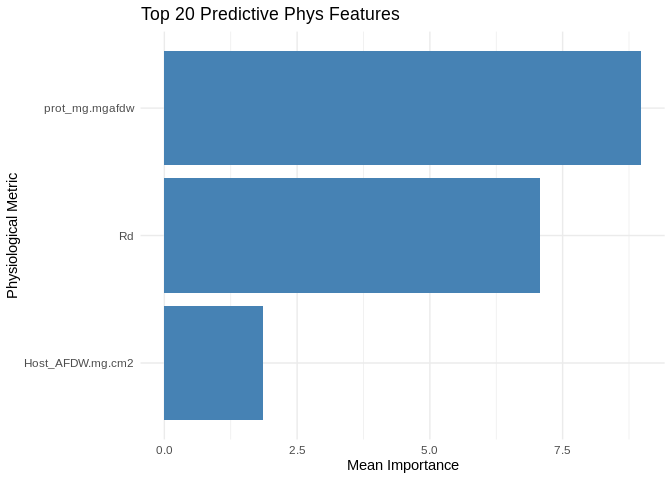
Protein was most predictive of expression, with respiration also highly predictive. Interestingly, biomass did not contribute much!

None of the gene PCs were well-predicted by phenotype, with the highest R² value sitting at 0.177 (~18% of variance in the PCs explained by phenotype).

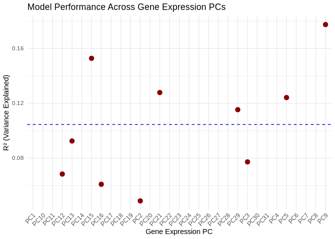Also, most of the expression PCs (21/31) had NA R² values, which I believe is related to low variance in the phenotype metrics, particularly the protein phenotype

> apply(merged_pcs, 2, var)

      PC1       PC2       PC3       PC4       PC5       PC6       PC7       PC8       PC9      PC10      PC11      PC12      PC13      PC14      PC15      PC16      PC17 
5801.1357 2808.7631 2370.6702 1990.1140 1760.0861 1627.7522 1317.6404 1274.2452 1078.4045 1034.5725  976.4311  937.5277  891.5255  796.3490  779.2450  699.0609  676.0976 
     PC18      PC19      PC20      PC21      PC22      PC23      PC24      PC25      PC26      PC27      PC28      PC29      PC30      PC31 
 650.9711  620.9733  606.8573  591.2129  575.7182  550.6815  528.1735  519.2895  506.3591  474.2105  467.2894  454.2832  436.9429  423.9563

> apply(phys_selection, 2, var)

Host_AFDW.mg.cm2   prot_mg.mgafdw               Rd 
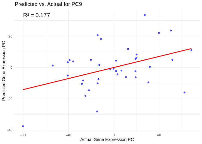
      0.33627626       0.01063323       0.03545622

We can look at model performance for specific expression PCs. For example, here’s PC9, which is the best-predicted PC (highest R² value)

We can also look at the top miRNA/genes associated with it. This was interesting because there is an miRNA that pops out (Cluster_4034)!

## # A tibble: 20 × 3
## # Groups:   Merged_PC [1]
##    gene_miRNA   Merged_PC Loading
##    <chr>        <chr>       <dbl>
##  1 FUN_023262   PC9       -0.0227
##  2 FUN_016918   PC9        0.0198
##  3 FUN_007014   PC9       -0.0194
##  4 FUN_031632   PC9        0.0192
##  5 FUN_035523   PC9        0.0188
##  6 FUN_041996   PC9        0.0188
##  7 FUN_006731   PC9       -0.0186
##  8 FUN_022897   PC9       -0.0185
##  9 FUN_043835   PC9        0.0184
## 10 FUN_004465   PC9        0.0183
## 11 FUN_014188   PC9       -0.0183
## 12 FUN_034114   PC9       -0.0181
## 13 FUN_024741   PC9       -0.0181
## 14 FUN_006446   PC9       -0.0179
## 15 FUN_018629   PC9       -0.0178
## 16 FUN_013857   PC9       -0.0178
## 17 Cluster_4034 PC9        0.0176
## 18 FUN_039308   PC9       -0.0175
## 19 FUN_012117   PC9        0.0175
## 20 FUN_000459   PC9       -0.0174

Code copied below in case of file path changes:

Inputs:

RNA counts matrix (raw): ../output/02.20-D-Apul-RNAseq-alignment-HiSat2/apul-gene_count_matrix.csv
sRNA/miRNA counts matrix (raw): ../output/03.10-D-Apul-sRNAseq-expression-DESeq2/Apul_miRNA_ShortStack_counts_formatted.txt
sample metadata: ../../M-multi-species/data/rna_metadata.csv
physiological data: https://github.com/urol-e5/timeseries/raw/refs/heads/master/time_series_analysis/Output/master_timeseries.csv

Note that I’ll start by using phenotype (e.g. biomass, respiration) as the predictor, which is suitable for understanding how external factors drive gene expression changes.

If, instead, we wanted to build some sort of predictive model, where gene expression could be used to predict phenotype, we could switch so that gene counts are used as the predictors.

Load libraries

library(tidyverse)
library(ggplot2)
library(DESeq2)
library(igraph)
library(psych)
library(tidygraph)
library(ggraph)
library(WGCNA)
library(edgeR)
library(reshape2)
library(ggcorrplot)
library(corrplot)
library(rvest)
library(purrr)
library(pheatmap)
library(glmnet)
library(caret)
library(factoextra)
library(vegan)
library(ggfortify)

Load and prep data

Load in count matrices for RNAseq.

# raw gene counts data (will filter and variance stabilize)
Apul_genes <- read_csv("../output/02.20-D-Apul-RNAseq-alignment-HiSat2/apul-gene_count_matrix.csv")
Apul_genes <- as.data.frame(Apul_genes)

# format gene IDs as rownames (instead of a column)
rownames(Apul_genes) <- Apul_genes$gene_id
Apul_genes <- Apul_genes%>%select(!gene_id)


# load and format metadata
metadata <- read_csv("../../M-multi-species/data/rna_metadata.csv")%>%select(AzentaSampleName, ColonyID, Timepoint) %>%
  filter(grepl("ACR", ColonyID))
metadata$Sample <- paste(metadata$AzentaSampleName, metadata$ColonyID, metadata$Timepoint, sep = "_")

colonies <- unique(metadata$ColonyID)

# Load physiological data
phys<-read_csv("https://github.com/urol-e5/timeseries/raw/refs/heads/master/time_series_analysis/Output/master_timeseries.csv")%>%filter(colony_id_corr %in% colonies)%>%
  select(colony_id_corr, species, timepoint, site, Host_AFDW.mg.cm2, Sym_AFDW.mg.cm2, Am, AQY, Rd, Ik, Ic, calc.umol.cm2.hr, cells.mgAFDW, prot_mg.mgafdw, Ratio_AFDW.mg.cm2, Total_Chl, Total_Chl_cell, cre.umol.mgafdw)
# format timepoint
phys$timepoint <- gsub("timepoint", "TP", phys$timepoint)
#add column with full sample info
phys <- merge(phys, metadata, by.x = c("colony_id_corr", "timepoint"), by.y = c("ColonyID", "Timepoint")) %>%
  select(-AzentaSampleName)
  

#add site information into metadata 
metadata$Site<-phys$site[match(metadata$ColonyID, phys$colony_id_corr)]


# Rename gene column names to include full sample info (as in miRNA table)
colnames(Apul_genes) <- metadata$Sample[match(colnames(Apul_genes), metadata$AzentaSampleName)]

# raw miRNA counts (will filter and variance stabilize)
Apul_miRNA <- read.table(file = "../output/03.10-D-Apul-sRNAseq-expression-DESeq2/Apul_miRNA_ShortStack_counts_formatted.txt", header = TRUE, sep = "\t", check.names = FALSE)

Counts filtering

Ensure there are no genes or miRNAs with 0 counts across all samples.

nrow(Apul_genes)

Apul_genes_filt<-Apul_genes %>%
     mutate(Total = rowSums(.[, 1:40]))%>%
    filter(!Total==0)%>%
    dplyr::select(!Total)

nrow(Apul_genes_filt)

# miRNAs
nrow(Apul_miRNA)

Apul_miRNA_filt<-Apul_miRNA %>%
     mutate(Total = rowSums(.[, 1:40]))%>%
    filter(!Total==0)%>%
    dplyr::select(!Total)

nrow(Apul_miRNA_filt)

Removing genes with only 0 counts reduced number from 44371 to 35869. Retained all 51 miRNAs.

Will not be performing pOverA filtering for now, since LM should presumabily incorporate sample representation

Physiology filtering

Run PCA on physiology data to see if there are phys outliers

Export data for PERMANOVA test.

test<-as.data.frame(phys)
test<-test[complete.cases(test), ]

Build PERMANOVA model.

scaled_test <-prcomp(test%>%select(where(is.numeric)), scale=TRUE, center=TRUE)
fviz_eig(scaled_test)

# scale data
vegan <- scale(test%>%select(where(is.numeric)))

# PerMANOVA 
permanova<-adonis2(vegan ~ timepoint*site, data = test, method='eu')
permanova

pca1<-ggplot2::autoplot(scaled_test, data=test, frame.colour="timepoint", loadings=FALSE,  colour="timepoint", shape="site", loadings.label.colour="black", loadings.colour="black", loadings.label=FALSE, frame=FALSE, loadings.label.size=5, loadings.label.vjust=-1, size=5) + 
  geom_text(aes(x = PC1, y = PC2, label = paste(colony_id_corr, timepoint)), vjust = -0.5)+
  theme_classic()+
   theme(legend.text = element_text(size=18), 
         legend.position="right",
        plot.background = element_blank(),
        legend.title = element_text(size=18, face="bold"), 
        axis.text = element_text(size=18), 
        axis.title = element_text(size=18,  face="bold"));pca1

Remove ACR-173, timepoint 3 sample from analysis. This is Azenta sample 1B2.

Apul_genes_filt <- Apul_genes_filt %>%
  select(!`1B2_ACR-173_TP3`)

Apul_miRNA_filt <- Apul_miRNA_filt %>%
  select(!`1B2_ACR-173_TP3`)

metadata <- metadata %>%
  filter(Sample != "1B2_ACR-173_TP3")

We also do not have phys data for colony 1B9 ACR-265 at TP4, so I’ll remove that here as well.

Apul_genes_filt <- Apul_genes_filt%>%
  select(!`1B9_ACR-265_TP4`)

Apul_miRNA_filt <- Apul_miRNA_filt%>%
  select(!`1B9_ACR-265_TP4`)

metadata <- metadata %>%
  filter(Sample != "1B9_ACR-265_TP4")

Assign metadata and arrange order of columns

Order metadata the same as the column order in the gene matrix.

list<-colnames(Apul_genes_filt)
list<-as.factor(list)

metadata$Sample<-as.factor(metadata$Sample)

# Re-order the levels
metadata$Sample <- factor(as.character(metadata$Sample), levels=list)
# Re-order the data.frame
metadata_ordered <- metadata[order(metadata$Sample),]
metadata_ordered$Sample

# Make sure the miRNA colnames are also in the same order as the gene colnames
Apul_miRNA_filt <- Apul_miRNA_filt[, colnames(Apul_genes_filt)]

Metadata and gene count matrix are now ordered the same.

Conduct variance stabilized transformation

VST should be performed on our two input datasets (gene counts and miRNA counts) separately

Genes:

#Set DESeq2 design
dds_genes <- DESeqDataSetFromMatrix(countData = Apul_genes_filt,
                              colData = metadata_ordered,
                              design = ~Timepoint+ColonyID)

Check size factors.

SF.dds_genes <- estimateSizeFactors(dds_genes) #estimate size factors to determine if we can use vst  to transform our data. Size factors should be less than 4 for us to use vst
print(sizeFactors(SF.dds_genes)) #View size factors

all(sizeFactors(SF.dds_genes)) < 4

All size factors are less than 4, so we can use VST transformation.

vsd_genes <- vst(dds_genes, blind=TRUE) #apply a variance stabilizing transformation to minimize effects of small counts and normalize with respect to library size
vsd_genes <- assay(vsd_genes)
head(vsd_genes, 3) #view transformed gene count data for the first three genes in the dataset.

miRNA:

#Set DESeq2 design
dds_miRNA <- DESeqDataSetFromMatrix(countData = Apul_miRNA_filt,
                              colData = metadata_ordered,
                              design = ~Timepoint+ColonyID)

Check size factors.

SF.dds_miRNA <- estimateSizeFactors(dds_miRNA) #estimate size factors to determine if we can use vst  to transform our data. Size factors should be less than 4 for us to use vst
print(sizeFactors(SF.dds_miRNA)) #View size factors

all(sizeFactors(SF.dds_miRNA)) < 4

All size factors are less than 4, so we can use VST transformation.

vsd_miRNA <- varianceStabilizingTransformation(dds_miRNA, blind=TRUE) #apply a variance stabilizing transformation to minimize effects of small counts and normalize with respect to library size. Using varianceStabilizingTransformation() instead of vst() because few input genes
vsd_miRNA <- assay(vsd_miRNA)
head(vsd_miRNA, 3) #view transformed gene count data for the first three genes in the dataset.

Combine counts data

# Extract variance stabilized counts as dataframes
# want samples in rows, genes/miRNAs in columns
vsd_genes <- as.data.frame(t(vsd_genes))
vsd_miRNA <- as.data.frame(t(vsd_miRNA))

# Double check the row names (sample names) are in same order
rownames(vsd_genes) == rownames(vsd_miRNA)

# Combine vst gene counts and vst miRNA counts by rows (sample names)
vsd_merged <- cbind(vsd_genes, vsd_miRNA)

Feature selection

Genes + miRNA

We have a large number of genes, so we’ll reduce dimensionality using PCA. Note that, since we only have a few phenotypes of interest, we don’t need to reduce this dataset

First need to remove any genes/miRNA that are invariant

vsd_merged_filt <- vsd_merged[, apply(vsd_merged, 2, var) > 0]

ncol(vsd_merged)
ncol(vsd_merged_filt)

colnames(vsd_merged[, apply(vsd_merged, 2, var) == 0])

Removed 74 invariant genes. I was worried we lost miRNA, but it looks like everything removed was a gene (prefix “FUN”)!

Reduce dimensionality (genes+miRNA)

# Perform PCA on gene+miRNA expression matrix
pca_merged <- prcomp(vsd_merged_filt, scale. = TRUE)

# Select top PCs that explain most variance (e.g., top 50 PCs)
explained_var <- summary(pca_merged)$importance[2, ]  # Cumulative variance explained
num_pcs <- min(which(cumsum(explained_var) > 0.95))  # Keep PCs that explain 95% variance

merged_pcs <- as.data.frame(pca_merged$x[, 1:num_pcs])  # Extract selected PCs

dim(merged_pcs)

We have 27 gene/miRNA expression PCs

Genes only

To investigate gene expression separately from miRNA expression, reduce dimensionality of genes alone.

Remove any genes that are invariant

vsd_genes_filt <- vsd_genes[, apply(vsd_genes, 2, var) > 0]

ncol(vsd_genes)
ncol(vsd_genes_filt)

Removed 74 invariant genes.

Reduce dimensionality

# Perform PCA on gene expression matrix
pca_genes <- prcomp(vsd_genes_filt, scale. = TRUE)

# Select top PCs that explain most variance (e.g., top 50 PCs)
explained_var_genes <- summary(pca_genes)$importance[2, ]  # Cumulative variance explained
num_pcs_genes <- min(which(cumsum(explained_var_genes) > 0.95))  # Keep PCs that explain 95% variance

genes_pcs <- as.data.frame(pca_genes$x[, 1:num_pcs_genes])  # Extract selected PCs

dim(genes_pcs)

Physiological metrics

Select physiological metrics of interest. For now we’ll focus on biomass (“Host_AFDW.mg.cm2”), protein (“prot_mg.mgafdw”), and respiration (“Rd”). These are all metrics of host energy storage and expenditure.

# Assign sample IDs to row names
rownames(phys) <- phys$Sample

# Select metrics
phys_selection <- phys %>% select(Host_AFDW.mg.cm2, prot_mg.mgafdw, Rd)

# Make sure the phys rownames are in the same order as the gene/miRNA rownames
phys_selection <- phys_selection[rownames(merged_pcs),]

Phenotype to predict gene/miRNA expression

The model

Train elastic models to predict gene expression PCs from phys data.

train_models <- function(response_pcs, predictor_pcs) {
  models <- list()
  
  for (pc in colnames(response_pcs)) {
    y <- response_pcs[[pc]]  # Gene expression PC
    X <- as.matrix(predictor_pcs)  # Phys as predictors
    
    # Train elastic net model (alpha = 0.5 for mix of LASSO & Ridge)
    model <- cv.glmnet(X, y, alpha = 0.5)
    
    models[[pc]] <- model
  }
  
  return(models)
}

# Train models predicting gene expression PCs from phys data
models <- train_models(merged_pcs, phys_selection)

Extract feature importance.

get_feature_importance <- function(models) {
  importance_list <- lapply(models, function(model) {
    coefs <- as.matrix(coef(model, s = "lambda.min"))[-1, , drop = FALSE]  # Convert to regular matrix & remove intercept
    
    # Convert to data frame
    coefs_df <- data.frame(Feature = rownames(coefs), Importance = as.numeric(coefs))
    
    return(coefs_df)
  })
  
  # Combine feature importance across all predicted gene PCs
  importance_df <- bind_rows(importance_list) %>%
    group_by(Feature) %>%
    summarize(MeanImportance = mean(abs(Importance)), .groups = "drop") %>%
    arrange(desc(MeanImportance))
  
  return(importance_df)
}

feature_importance <- get_feature_importance(models)
head(feature_importance, 20)  # Top predictive phys features

Evaluate performance.

evaluate_model_performance <- function(models, response_pcs, predictor_pcs) {
  results <- data.frame(PC = colnames(response_pcs), R2 = NA)
  
  for (pc in colnames(response_pcs)) {
    y <- response_pcs[[pc]]
    X <- as.matrix(predictor_pcs)
    
    model <- models[[pc]]
    preds <- predict(model, X, s = "lambda.min")
    
    R2 <- cor(y, preds)^2  # R-squared metric
    results[results$PC == pc, "R2"] <- R2
  }
  
  return(results)
}

performance_results <- evaluate_model_performance(models, merged_pcs, phys_selection)
summary(performance_results$R2)

Results

Plot results.

# Select top 20 predictive phys features
top_features <- feature_importance %>% top_n(20, MeanImportance)

# Plot
ggplot(top_features, aes(x = reorder(Feature, MeanImportance), y = MeanImportance)) +
  geom_bar(stat = "identity", fill = "steelblue") +
  coord_flip() +  # Flip for readability
  theme_minimal() +
  labs(title = "Top 20 Predictive Phys Features",
       x = "Physiological Metric",
       y = "Mean Importance")

ggplot(performance_results, aes(x = PC, y = R2)) +
  geom_point(color = "darkred", size = 3) +
  geom_hline(yintercept = mean(performance_results$R2, na.rm = TRUE), linetype = "dashed", color = "blue") +
  theme_minimal() +
  labs(title = "Model Performance Across Gene Expression PCs",
       x = "Gene Expression PC",
       y = "R² (Variance Explained)") +
  theme(axis.text.x = element_text(angle = 45, hjust = 1))  # Rotate labels

Keep in mind that, while we ran the model with physiological predictors, we’re really interested in the genes/miRNA associated with these predictors

View components associated with gene/miRNA PCs

# Get the PCA rotation (loadings) matrix from the original gene/miRNA PCA
merged_loadings <- pca_merged$rotation  # Each column corresponds to a PC

# Convert to data frame and reshape for plotting
merged_loadings_df <- as.data.frame(merged_loadings) %>%
  rownames_to_column(var = "gene_miRNA") %>%
  pivot_longer(-gene_miRNA, names_to = "Merged_PC", values_to = "Loading")

# View top CpGs contributing most to each PC
top_genes <- merged_loadings_df %>%
  group_by(Merged_PC) %>%
  arrange(desc(abs(Loading))) %>%
  slice_head(n = 20)  # Select top 10 CpGs per PC

print(top_genes)

View top 20 miRNA/genes associated with PC9 (the PC with the highest R^2)

print(top_genes%>%filter(Merged_PC=="PC9"))

Interesting, there’s an miRNA in there!

View predicted vs actual gene expression values to evaluate model.

# Choose a gene expression PC to visualize (e.g., the most predictable one)
best_pc <- performance_results$PC[which.max(performance_results$R2)]

# Extract actual and predicted values for that PC
actual_values <- merged_pcs[[best_pc]]
predicted_values <- predict(models[[best_pc]], as.matrix(phys_selection), s = "lambda.min")

# Create data frame
prediction_df <- data.frame(
  Actual = actual_values,
  Predicted = predicted_values
)

# Scatter plot with regression line
ggplot(prediction_df, aes(x = Actual, y = lambda.min)) +
  geom_point(color = "blue", alpha = 0.7) +
  geom_smooth(method = "lm", color = "red", se = FALSE) +
  theme_minimal() +
  labs(title = paste("Predicted vs. Actual for", best_pc),
       x = "Actual Gene Expression PC",
       y = "Predicted Gene Expression PC") +
  annotate("text", x = min(actual_values), y = max(predicted_values), 
           label = paste("R² =", round(max(performance_results$R2, na.rm=TRUE), 3)), 
           hjust = 0, color = "black", size = 5)
## `geom_smooth()` using formula = 'y ~ x'