Rscript 26.2-ElasticNet-scaling.R \
"ortholog_gene_counts_path.csv" \
"miRNA_counts_path.txt" \
"lncRNA_counts_path.txt" \
"methylation_matrix_path.tsv" \
"metadata_file_path.csv" \
"output_dir_path" \
"list_samples_to_exclude" \   # (comma-separated string like "s1,s2")
0.5 \   # alpha value for EN model (optional, default 0.5)
25 \    # Num. replicates for first bootstrapping round (optional, default 50)
50 \    # Num. replicates for second bootstrapping round (after reducing to only well-predicted genes) (optional, default 50)
0.5 # r^2 threshold for "well-predicted" genes (optional, default 0.5)Will be using the Elastic Net script I made a few weeks ago: timeseries/M-multi-species/scripts/26.2-ElasticNet-scaling.R (link)
Took some more time to fix different formatting problems that arose when inputting new matrices, but should be plug-and-play now!
To use, run following command (I’ve needed to do so in a conda environment when working in Raven):
Importantly, its now set up to run on input gene sets of orthologs, which may have two “name” columns, one for ortholog ID and one for gene ID. IT will use the ortholog ID instead of gene ID )since some genes are included in multiple orthologs). That’s why line 199 reads:
genes <- as.data.frame(read.csv(genes_file)) %>% select(-gene_id)
If you’re instead working with just genes (not orthologs), you’d want to comment out this line.
Now, rerunning with new inputs: Using gene set of orthorlogs involved in biomineralization, and GbM for the WGBS predictor input
Output directories:
26.2-ElasticNet-scaling-GbM
26.2-ElasticNet-scaling-GbM-noise
Apul
(r_enet_rscript) shedurkin@raven:~/timeseries_molecular/M-multi-species/scripts$ Rscript 26.2-ElasticNet-scaling.R \
"https://raw.githubusercontent.com/urol-e5/timeseries-molecular-calcification/refs/heads/main/M-multi-species/output/33-biomin-pathway-counts/apul_biomin_counts.csv" \
"https://github.com/urol-e5/timeseries_molecular/raw/refs/heads/main/M-multi-species/output/10.1-format-miRNA-counts-updated/Apul_miRNA_counts_formatted_updated.txt" \
"https://gannet.fish.washington.edu/v1_web/owlshell/bu-github/timeseries_molecular/D-Apul/output/31.5-Apul-lncRNA-discovery/lncRNA_counts.clean.filtered.txt" \
"https://raw.githubusercontent.com/urol-e5/timeseries-molecular-calcification/refs/heads/main/D-Apul/output/40-Apul-Gene-Methylation/Apul-gene-methylation_75pct.tsv" \
"../../M-multi-species/data/rna_metadata.csv" \
"../output/26.2-ElasticNet-scaling-GbM" \
"ACR-225-TP1" \
0.5 \
25 \
50 \
0.5
Then want to generate a “fake” predictor set of just noise. For now I’ll choose to (a) use a fully randomized predictor set, instead of “spiking” noise into the real data, and (b) to generate the random data empirically
make_noise_empirical_safe <- function(X) {

  X_noise <- apply(X, 2, function(col) {
    sample(col, length(col), replace = TRUE)
  })

  # Ensure row/col names preserved
  colnames(X_noise) <- colnames(X)
  X_noise[,1] <- X[,1]

  # Fix rows that become all-zero
  zero_rows <- which(rowSums(X_noise > 0) == 0)
  if (length(zero_rows) > 0) {
    for (i in zero_rows) {
      # Give the row a single small positive value
      # Put it in a random column
      j <- sample(seq_len(ncol(X_noise)), 1)
      X_noise[i, j] <- 1
    }
  }

  return(X_noise)
}

miRNA_noise <- make_noise_empirical(miRNA)
lncRNA_noise <- make_noise_empirical(lncRNA)
WGBS_noise <- make_noise_empirical(WGBS)

write.table(mirna_noise, "./M-multi-species/output/26.2-ElasticNet-scaling-GbM-noise/mirna_empirical_noise.txt", row.names=FALSE, sep="\t")
write.table(lncrna_noise, "./M-multi-species/output/26.2-ElasticNet-scaling-GbM-noise/lncrna_empirical_noise.txt", row.names=FALSE, sep="\t")
write.csv(wgbs_noise, "./M-multi-species/output/26.2-ElasticNet-scaling-GbM-noise/wgbs_empirical_noise.csv", row.names=FALSE)(r_enet_rscript) shedurkin@raven:~/timeseries_molecular/M-multi-species/scripts$ Rscript 26.2-ElasticNet-scaling.R \
"https://raw.githubusercontent.com/urol-e5/timeseries-molecular-calcification/refs/heads/main/M-multi-species/output/33-biomin-pathway-counts/apul_biomin_counts.csv" \
"../output/26.2-ElasticNet-scaling-GbM-noise/mirna_empirical_noise.txt" \
"../output/26.2-ElasticNet-scaling-GbM-noise/lncrna_empirical_noise.txt" \
"../output/26.2-ElasticNet-scaling-GbM-noise/wgbs_empirical_noise.csv" \
"../../M-multi-species/data/rna_metadata.csv" \
"../output/26.2-ElasticNet-scaling-GbM-noise" \
"ACR-225-TP1" \
0.5 \
25 \
50 \
0.5As with CpG site methylation, running the EN with GbM methylation as one of the predictors and empirical noise as the gene set still results in a non-functional model, confirming the EN is identifying “real” patterns in our data (not just noise related to large data set/multiple testing). Nice!
Peve
POR-69-TP3) and WGBS counts (POR-73-TP2). Also exclude POR-236-TP2, which has 0 counts for all miRNA. This makes it both biologically uninformative and creates NA values during scaling. I’m also going to exclude the following samples, which have almost entirely 0 counts for miRNA, suggesting a sample processing/sequencing issue: POR-74-TP4, POR-262-TP4, POR-262-TP3, and POR-69-TP2.
(r_enet_rscript) shedurkin@raven:~/timeseries_molecular/M-multi-species/scripts$ Rscript 26.2-ElasticNet-scaling.R \
"https://raw.githubusercontent.com/urol-e5/timeseries-molecular-calcification/refs/heads/main/M-multi-species/output/33-biomin-pathway-counts/peve_biomin_counts.csv" \
"https://github.com/urol-e5/timeseries_molecular/raw/refs/heads/main/M-multi-species/output/10.1-format-miRNA-counts-updated/Peve_miRNA_counts_formatted_updated.txt" \
"https://gannet.fish.washington.edu/v1_web/owlshell/bu-github/timeseries_molecular/E-Peve/output/12-Peve-lncRNA-discovery/lncRNA_counts.clean.filtered.txt" \
"https://raw.githubusercontent.com/urol-e5/timeseries-molecular-calcification/refs/heads/main/E-Peve/output/15-Peve-Gene-Methylation/Peve-gene-methylation_75pct.tsv" \
"../../M-multi-species/data/rna_metadata.csv" \
"../output/26.2-ElasticNet-scaling-GbM" \
"POR-69-TP2,POR-69-TP3,POR-73-TP2,POR-74-TP4,POR-236-TP2,POR-262-TP4,POR-262-TP3" \
0.5 \
25 \
50 \
0.5
Ptuh
Exclude: “POC-201-TP3,POC-222-TP2,POC-255-TP4,POC-259-TP3,POC-259-TP4,POC-42-TP1,POC-42-TP3”
(r_enet_rscript) shedurkin@raven:~/timeseries_molecular/M-multi-species/scripts$ Rscript 26.2-ElasticNet-scaling.R \
"https://raw.githubusercontent.com/urol-e5/timeseries-molecular-calcification/refs/heads/main/M-multi-species/output/33-biomin-pathway-counts/ptua_biomin_counts.csv" \
"https://github.com/urol-e5/timeseries_molecular/raw/refs/heads/main/M-multi-species/output/10.1-format-miRNA-counts-updated/Ptuh_miRNA_counts_formatted_updated.txt" \
"https://raw.githubusercontent.com/urol-e5/timeseries_molecular/refs/heads/main/F-Ptua/output/06-Ptua-lncRNA-discovery/lncRNA_counts.clean.filtered.txt" \
"https://raw.githubusercontent.com/urol-e5/timeseries-molecular-calcification/refs/heads/main/F-Ptua/output/09-Ptua-Gene-Methylation/Ptua-gene-methylation_75pct.tsv" \
"../../M-multi-species/data/rna_metadata.csv" \
"../output/26.2-ElasticNet-scaling-GbM" \
"POC-201-TP3,POC-222-TP2,POC-255-TP4,POC-259-TP3,POC-259-TP4,POC-42-TP1,POC-42-TP3" \
0.5 \
25 \
50 \
0.5
Plotting
library(dplyr)Warning: package 'dplyr' was built under R version 4.2.3library(ggplot2)
library(tidyr)Warning: package 'tidyr' was built under R version 4.2.3library(purrr)df_ACR <- read.csv("https://github.com/urol-e5/timeseries_molecular/raw/refs/heads/main/M-multi-species/output/26.2-ElasticNet-scaling-GbM/Apul_top_predictors.csv", header=TRUE)
df_POR <- read.csv("https://github.com/urol-e5/timeseries_molecular/raw/refs/heads/main/M-multi-species/output/26.2-ElasticNet-scaling-GbM/Peve_top_predictors.csv", header=TRUE)
df_POC <- read.csv("https://github.com/urol-e5/timeseries_molecular/raw/refs/heads/main/M-multi-species/output/26.2-ElasticNet-scaling-GbM/Ptuh_top_predictors.csv", header=TRUE)get_topN <- function(df, N, species_name) {
df %>%
group_by(Feature) %>%
slice_max(order_by = MeanImportance, n = N, with_ties = FALSE) %>%
mutate(Species = species_name)
}
topN <- bind_rows(
get_topN(df_ACR, N = 10, species_name = "ACR"),
get_topN(df_POR, N = 10, species_name = "POR"),
get_topN(df_POC, N = 10, species_name = "POC")
)
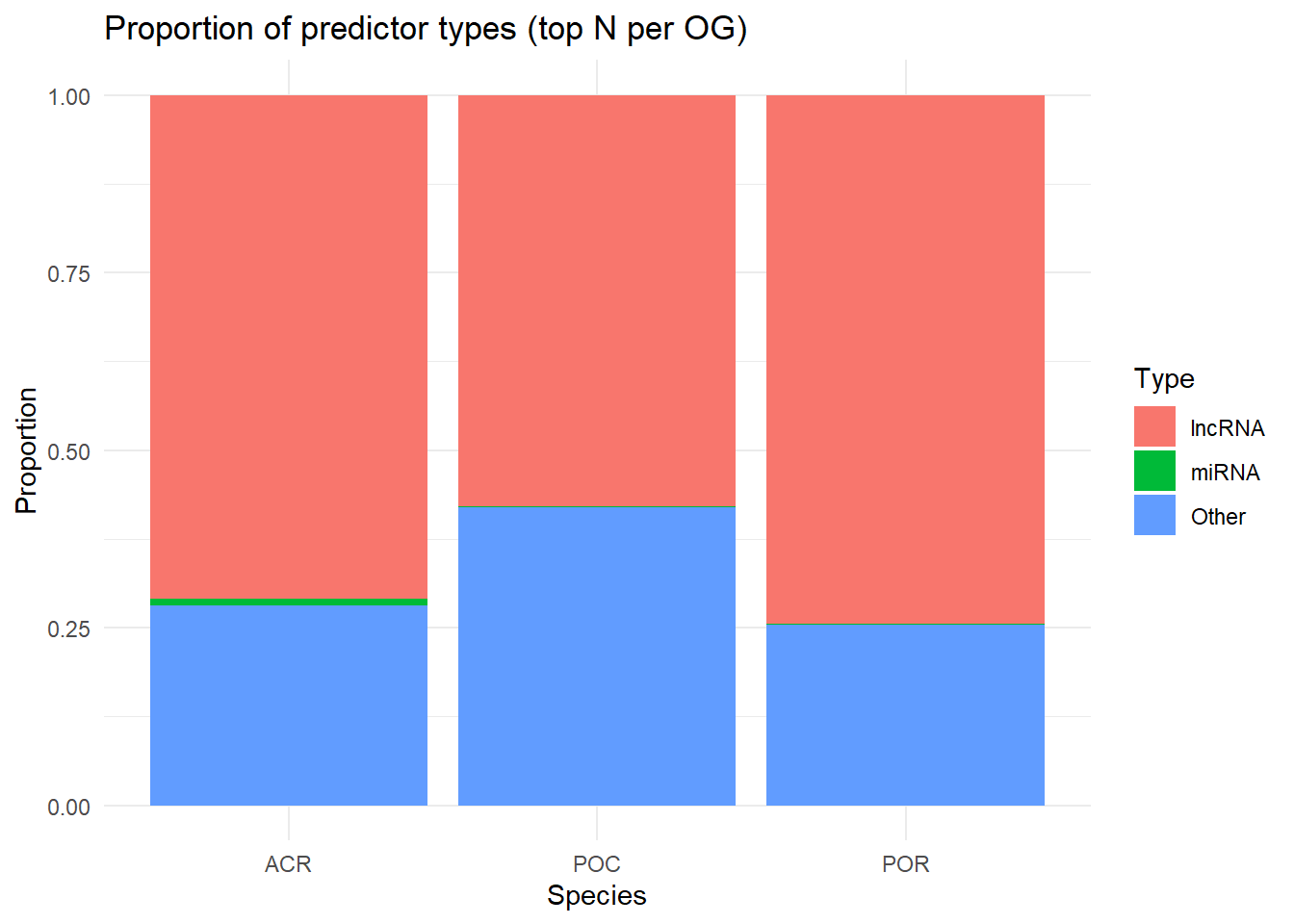
species_prop <- topN %>%
group_by(Species, Type) %>%
summarize(n = n(), .groups="drop") %>%
group_by(Species) %>%
mutate(prop = n / sum(n))
ggplot(species_prop, aes(x = Species, y = prop, fill = Type)) +
geom_col() +
theme_minimal() +
labs(title = "Proportion of predictor types (top N per OG)",
y = "Proportion")