Correcting CIRCOES plot generated here for DDE manuscript. Old plot shows which targets are orthologus genes (present in more than one species) – I need the plot to be showing orthologs that are targeted by miR-100 in more than one species.
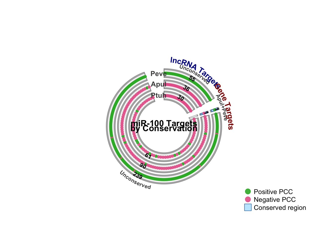
TLDR: Only one orthogroup is targeted by miR-100 in more than one species, targeted in A. pulchra and P. evermanni. This ortholg is not functionally annotated.
Updated plot showing this conservation is stored here
Load libraries
library(dplyr)
Attaching package: 'dplyr'
The following objects are masked from 'package:stats':

    filter, lag
The following objects are masked from 'package:base':

    intersect, setdiff, setequal, union
========================================
circlize version 0.4.17
CRAN page: https://cran.r-project.org/package=circlize
Github page: https://github.com/jokergoo/circlize
Documentation: https://jokergoo.github.io/circlize_book/book/

If you use it in published research, please cite:
Gu, Z. circlize implements and enhances circular visualization
  in R. Bioinformatics 2014.

This message can be suppressed by:
  suppressPackageStartupMessages(library(circlize))
========================================
Rows: 52280 Columns: 3
── Column specification ────────────────────────────────────────────────────────
Delimiter: "\t"
chr (3): Orthogroup, Species, Proteins

ℹ Use `spec()` to retrieve the full column specification for this data.
ℹ Specify the column types or set `show_col_types = FALSE` to quiet this message.
Add column showing whether a given orthogroup contains proteins from all species or only a subset.
# Standardize species names for simplicityh_ortho <- h_ortho %>%mutate(simple_species =case_when(grepl("Apulchra", Species) ~"apul",grepl("Porites_evermanni", Species) ~"peve",grepl("Pocillopora_meandrina", Species) ~"ptuh",TRUE~"other" ) )# Summarize species presence per orthogrouph_ortho_summary <- h_ortho %>%group_by(Orthogroup) %>%summarise(type =case_when(all(c("apul", "peve", "ptuh") %in% simple_species) ~"three_way",all(c("apul", "peve") %in% simple_species) &!("ptuh"%in% simple_species) ~"apul_peve",all(c("apul", "ptuh") %in% simple_species) &!("peve"%in% simple_species) ~"apul_ptuh",all(c("peve", "ptuh") %in% simple_species) &!("apul"%in% simple_species) ~"peve_ptuh",TRUE~"other" ),.groups ="drop" )# Join back to originalh_ortho <- h_ortho %>%left_join(h_ortho_summary, by ="Orthogroup")
Huh, looks like Hollie’s analysis only outputs orthogroups which contain at least one protein from each species
Hmm, so it turns out there’s only one orthogroup that is targeted by miR-100 in more than one species – the orthogroup contains both FUN_035913 in A. pulchra and Peve_00006734 in P. evermanni. On top of that, this single conserved target is also not functionally annotated (does not closely match any previously functionall described sequence – checked here). On the bright side, this conserved targeting shows up in the outputs of both Hollie’s and Steven’s ortholog analyses, so I don’t need to worry about reconciling/picking between divergent results.
This isn’t particularly useful/exciting, so I’m not sure its even worth displaying in the planned plot, but I’ll go ahead and do it for posterity.
Plot
# Set margins to allow room for outer labelspar(mar =c(2, 2, 4, 2))# Define segments for compact version - unconserved targets share same segmentsegment_info_v3 <-list(# lncRNA segments (left half of circle)"lnc_all_3"=list(label ="All 3",species =c("Apul", "Peve", "Ptuh"),ortho_conserv ="three_way",target_type ="lncRNA",conserved =TRUE ),"lnc_apul_peve"=list(label ="Apul+Peve",species =c("Apul", "Peve"),ortho_conserv ="apul_peve",target_type ="lncRNA",conserved =TRUE ),"lnc_peve_ptuh"=list(label ="Peve+Ptuh",species =c("Peve", "Ptuh"),ortho_conserv ="peve_ptuh",target_type ="lncRNA",conserved =TRUE ),"lnc_apul_ptuh"=list(label ="Apul+Ptuh",species =c("Apul", "Ptuh"),ortho_conserv ="apul_ptuh",target_type ="lncRNA",conserved =TRUE ),"lnc_unconserved"=list(label ="Unconserved",species =c("Apul", "Peve", "Ptuh"),ortho_conserv ="none",target_type ="lncRNA",conserved =FALSE ),# Gene segments (right half of circle)"gene_all_3"=list(label ="All 3",species =c("Apul", "Peve", "Ptuh"),ortho_conserv ="three_way",target_type ="gene",conserved =TRUE ),"gene_apul_peve"=list(label ="Apul+Peve",species =c("Apul", "Peve"),ortho_conserv ="apul_peve",target_type ="gene",conserved =TRUE ),"gene_peve_ptuh"=list(label ="Peve+Ptuh",species =c("Peve", "Ptuh"),ortho_conserv ="peve_ptuh",target_type ="gene",conserved =TRUE ),"gene_apul_ptuh"=list(label ="Apul+Ptuh",species =c("Apul", "Ptuh"),ortho_conserv ="apul_ptuh",target_type ="gene",conserved =TRUE ),"gene_unconserved"=list(label ="Unconserved",species =c("Apul", "Peve", "Ptuh"),ortho_conserv ="none",target_type ="gene",conserved =FALSE ))# Calculate segment sizes for v3 - unconserved segments need max across all speciescalc_segment_sizes_v3 <-function(data, segment_info) { sizes <-list()for (seg_name innames(segment_info)) { seg <- segment_info[[seg_name]]if (seg$ortho_conserv =="none") {# Unconserved: find the max count across all species max_n <-0for (sp in seg$species) { n <- data %>%filter(s_ortho_conserv =="none", species == sp, target_type == seg$target_type) %>%select(target) %>%distinct() %>%nrow() max_n <-max(max_n, n) } sizes[[seg_name]] <-max(max_n, 1) } else {# Conserved: filter by ortho type and target type n <- data %>%filter(s_ortho_conserv == seg$ortho_conserv, target_type == seg$target_type) %>%select(target) %>%distinct() %>%nrow() sizes[[seg_name]] <-max(n, 1) } }return(sizes)}# Create compact circos plot with overlapping unconserved targetscreate_circos_plot_v3 <-function(data) {# Species order (outer to inner): Peve (most), Apul, Ptuh (fewest) species_order <-c("Peve", "Apul", "Ptuh")# Calculate segment sizes seg_sizes <-calc_segment_sizes_v3(data, segment_info_v3)# Define sector order: lncRNA segments first, then gene segments lnc_segments <-c("lnc_all_3", "lnc_apul_peve", "lnc_peve_ptuh", "lnc_apul_ptuh", "lnc_unconserved") gene_segments <-c("gene_all_3", "gene_apul_peve", "gene_apul_ptuh", "gene_peve_ptuh", "gene_unconserved")# Filter to only segments with data lnc_segments <- lnc_segments[sapply(lnc_segments, function(s) { seg <- segment_info_v3[[s]]if (seg$ortho_conserv =="none") {nrow(data %>%filter(s_ortho_conserv =="none", target_type =="lncRNA")) >0 } else {nrow(data %>%filter(s_ortho_conserv == seg$ortho_conserv, target_type =="lncRNA")) >0 } })] gene_segments <- gene_segments[sapply(gene_segments, function(s) { seg <- segment_info_v3[[s]]if (seg$ortho_conserv =="none") {nrow(data %>%filter(s_ortho_conserv =="none", target_type =="gene")) >0 } else {nrow(data %>%filter(s_ortho_conserv == seg$ortho_conserv, target_type =="gene")) >0 } })]# All sectors in order all_sectors <-c(lnc_segments, gene_segments)if (length(all_sectors) ==0) {message("No data to plot")return(invisible(NULL)) }# Build xlims xlims <-list()for (seg_name in all_sectors) { xlims[[seg_name]] <-c(0, seg_sizes[[seg_name]]) }# Initialize circoscircos.clear()# Calculate gap degrees - larger gaps between lncRNA and gene halves n_lnc <-length(lnc_segments) n_gene <-length(gene_segments) n_total <- n_lnc + n_gene# Create gap vector: small gaps within each half, large gap between halves gap_degrees <-rep(3, n_total)if (n_lnc >0&& n_gene >0) { gap_degrees[n_lnc] <-10 gap_degrees[n_total] <-20 }circos.par(start.degree =90,gap.degree = gap_degrees,track.margin =c(0.02, 0.02),cell.padding =c(0.02, 0.1, 0.02, 0.1),canvas.xlim =c(-1.4, 1.4),canvas.ylim =c(-1.4, 1.4) )circos.initialize(factors =factor(all_sectors, levels = all_sectors),xlim =do.call(rbind, xlims[all_sectors]) )# Colors highlight_col <-rgb(0.6, 0.85, 1, 0.6) # Light blue for conserved no_highlight_col <-rgb(0.95, 0.95, 0.95, 1) # Light grey for unconserved pos_col <-rgb(0.2, 0.7, 0.2, 0.9) # Green for positive PCC neg_col <-rgb(0.9, 0.4, 0.6, 0.9) # Pink for negative PCC border_col <-rgb(0.3, 0.5, 0.7, 1) # Blue border# Create 3 tracks (one per species, outer to inner)for (sp_idx in1:3) { sp <- species_order[sp_idx]circos.track(factors =factor(all_sectors, levels = all_sectors),ylim =c(0, 1),track.height =0.15,bg.border ="grey60",bg.lwd =1.5,panel.fun =function(x, y) { sector_name <- CELL_META$sector.index seg <- segment_info_v3[[sector_name]]# For conserved segments, check if species is in the conservation group# For unconserved, all species appear but no highlightingif (seg$conserved) { sp_in_segment <- sp %in% seg$species } else { sp_in_segment <-TRUE# All species appear in unconserved segment }# Background colorif (seg$conserved && sp_in_segment) { bg_col <- highlight_col border <- border_col } elseif (sp_in_segment) { bg_col <- no_highlight_col border <-"grey60" } else { bg_col <-"white" border <-"grey80" }# Draw background rectanglecircos.rect( CELL_META$xlim[1], 0, CELL_META$xlim[2], 1,col = bg_col,border = border,lwd =1.5 )# Plot pointsif (seg$ortho_conserv =="none") {# Unconserved: each species plots its own targets seg_data <- data %>%filter(species == sp, s_ortho_conserv =="none", target_type == seg$target_type) %>%distinct(target, .keep_all =TRUE) } elseif (sp_in_segment) {# Conserved: filter by ortho type seg_data <- data %>%filter(species == sp, s_ortho_conserv == seg$ortho_conserv, target_type == seg$target_type) %>%distinct(target, .keep_all =TRUE) } else { seg_data <-data.frame() }if (nrow(seg_data) >0) { n_points <-nrow(seg_data)if (n_points ==1) { x_positions <- CELL_META$xlim[2] /2 } else { x_positions <-seq(0.5, CELL_META$xlim[2] -0.5, length.out = n_points) }for (i in1:n_points) { pt_col <-ifelse(seg_data$PCC_direction[i] >0, pos_col, neg_col)circos.points( x_positions[i], 0.5,col = pt_col,pch =21,bg = pt_col,cex =0.75 ) }# Add count label above the feature pointscircos.text(x =mean(x_positions),y =0.85,labels =as.character(n_points),facing ="bending.inside",niceFacing =TRUE,cex =0.75,col ="black",font =2 ) } } ) }# Add segment labels on the outsidefor (seg_name in all_sectors) { seg <- segment_info_v3[[seg_name]]circos.text(x =mean(xlims[[seg_name]]),y =1.8,sector.index = seg_name,track.index =1,labels = seg$label,facing ="bending.outside",niceFacing =TRUE,cex =0.7,font =2,col ="grey30" ) }# Add "lncRNA" and "Genes" labels for each halfif (n_lnc >0) { mid_lnc <- lnc_segments[ceiling(n_lnc /2)]circos.text(x =mean(xlims[[mid_lnc]]),y =2.5,sector.index = mid_lnc,track.index =1,labels ="lncRNA Targets",facing ="bending.outside",niceFacing =TRUE,cex =1.0,font =2,col ="darkblue" ) }if (n_gene >0) { mid_gene <- gene_segments[ceiling(n_gene /2)]circos.text(x =mean(xlims[[mid_gene]]),y =2.5,sector.index = mid_gene,track.index =1,labels ="Gene Targets",facing ="bending.outside",niceFacing =TRUE,cex =1.0,font =2,col ="darkred" ) }# Add title and species labels in the center (outer to inner: Peve, Apul, Ptuh)text(0, 0.04, "miR-100 Targets", font =2, cex =1.1, col ="black")text(0, -0.04, "by Conservation", font =2, cex =1.1, col ="black")text(-0.09, 0.9, "Peve", font =2, cex =0.9, col ="grey30")text(-0.09, 0.71, "Apul", font =2, cex =0.9, col ="grey30")text(-0.09, 0.53, "Ptuh", font =2, cex =0.9, col ="grey30")# Add legendlegend("bottomright",legend =c("Positive PCC", "Negative PCC", "Conserved region"),pch =c(21, 21, 22),pt.bg =c(pos_col, neg_col, highlight_col),col =c(pos_col, neg_col, border_col),pt.cex =c(1.5, 1.5, 2.2),bty ="n",cex =0.85 )circos.clear()}# Create the compact plotcreate_circos_plot_v3(data)
Note: 1 point is out of plotting region in sector 'lnc_unconserved',
track '1'.
Note: 1 point is out of plotting region in sector 'lnc_unconserved',
track '1'.
Note: 11 points are out of plotting region in sector 'lnc_unconserved',
track '1'.
Note: 1 point is out of plotting region in sector 'gene_apul_peve',
track '1'.
Note: 1 point is out of plotting region in sector 'gene_apul_peve',
track '1'.
Note: 9 points are out of plotting region in sector 'gene_apul_peve',
track '1'.
Note: 1 point is out of plotting region in sector 'gene_unconserved',
track '1'.
Note: 1 point is out of plotting region in sector 'gene_unconserved',
track '1'.
Note: 11 points are out of plotting region in sector
'gene_unconserved', track '1'.
Note: 1 point is out of plotting region in sector 'lnc_unconserved',
track '1'.
Note: 1 point is out of plotting region in sector 'lnc_unconserved',
track '1'.
Note: 14 points are out of plotting region in sector 'lnc_unconserved',
track '1'.
Note: 1 point is out of plotting region in sector 'gene_apul_peve',
track '1'.
Note: 1 point is out of plotting region in sector 'gene_apul_peve',
track '1'.
Note: 12 points are out of plotting region in sector 'gene_apul_peve',
track '1'.
# Save to pngpng("output/2026_04_08_DDE_plot_edits/s_orthos_circos_plot.png", width =2000, height =2000, res =300)create_circos_plot_v3(data)
Note: 1 point is out of plotting region in sector 'lnc_unconserved',
track '1'.
Note: 1 point is out of plotting region in sector 'lnc_unconserved',
track '1'.
Note: 11 points are out of plotting region in sector 'lnc_unconserved',
track '1'.
Note: 1 point is out of plotting region in sector 'gene_apul_peve',
track '1'.
Note: 1 point is out of plotting region in sector 'gene_apul_peve',
track '1'.
Note: 9 points are out of plotting region in sector 'gene_apul_peve',
track '1'.
Note: 1 point is out of plotting region in sector 'gene_unconserved',
track '1'.
Note: 1 point is out of plotting region in sector 'gene_unconserved',
track '1'.
Note: 11 points are out of plotting region in sector
'gene_unconserved', track '1'.
Note: 1 point is out of plotting region in sector 'lnc_unconserved',
track '1'.
Note: 1 point is out of plotting region in sector 'lnc_unconserved',
track '1'.
Note: 14 points are out of plotting region in sector 'lnc_unconserved',
track '1'.
Note: 1 point is out of plotting region in sector 'gene_apul_peve',
track '1'.
Note: 1 point is out of plotting region in sector 'gene_apul_peve',
track '1'.
Note: 12 points are out of plotting region in sector 'gene_apul_peve',
track '1'.