Implementing MACAU to identify differentially methylated loci (DMLs) in ceasmallr data based on parent treatment, while accounting for shared parentage. Note that, due to various package/version mismatches, I ended up using PQLSeq2 to run the MACAU model, rather than the original MACAU 2.0 R package.
For this initial attempt I generated a relatedness matrix the “easy” way, by simply assigning half-sib values to offspring based on parent IDs.
Full code at 11-diff-methyl-MACAU.Rmd
Results
Ran wilth all 32 offspring samples (low-coverage samples were not removed, to maximize sample size).
2148546 loci retained after filtering
Pedigree matrix (constructed from parent IDs)
MACAU run
sites into fit: 2148546
sites returned: 2148546 (100% survived fitting)
of those, converged: 1997127 (93%)
Treatment DMLs (FDR < 0.05): 799 (361 hyper, 438 hypo)
Interpretation/notes/next steps
I believe the test run here is most comparable to the DSS test DMLfit.multiFactor(BSobj, design = design, formula = ~ treatment + stage), which adjusts for lifestage but does not permit/account for an interaction effect between parental treatment and lifestage.
Applying the above DSS model fit to all samples identified 11,356 DMLs. This is more than 10X the number of significant DMLs identified as here, 799! Part of that is probably explained by the difference in # of sites tested (this MACAU work required an additional filter to remove invariant sites within treatment groups): when using all samples, 6,337,469 sites tested in DSS work; 2,148,546 sites tested in MACAU work.
However, the difference may also be explained in part by relatedness effects – DSS may have been identiying some treatment-related DMLs that are actually artifacts of shared parentage (pseudoreplication). I think that DMLs identified in both sets would be the most robust.
Keep in mind, however, that MACAU is unable to identify loci for which treatment effect Differs by stage, which DSS can answer using a ~treatment + stage + treatment:stage design.
I also have a concern about the way I’ve created the relatedness matrix here. Because all offspring were generated using within-treatment crosses (control M x contol F; exposed M x exposed F), by using parent IDs to generate the matrix, I’ve also nested relatedness and treatment. This is visible in the relatedness matrix heatmap, which shows 0 relatedness for all cross-treatment comparisons (i.e. all CxC and ExE comparisons are completely unrelated). The down-stream analysis problem becomes evident when looking at the h2 values of output DMLs. The vast majority (59/799, or ~7%) are either 0 (no variance explained by relatedness), 1 (all explained by relatedness), or NA. This is an indicator of covariate confounding – the treatment parameter and relatedness matrix are colinear by nature of the experimental design and matrix construction approach.
The fix should be conceptually straightforward, if a little annoying to implement. WGBS data is essentially modified WGS data – I can use WGBS data with a bisulfite-conversion-aware caller (e.g., Revelio) to call SNPs and then generate a relatedness matrix using GEMMA, as recommended in the MACAU user manual.
Code
Differential methylation analysis using MACAU, which has built-in functionality for incorporating informatin on population structure. This will help account for pseudoreplication in our ceasmallr samples stemming from shared parentage among the specimens.
As in 10-diff-methyl-DSS.Rmd and 10.1-diff-methyl-DSS-parents.Rmd, will need to run this .rmd using a .sh script on Klone (copy below for posterity)
#!/bin/bash
#SBATCH --account=srlab
#SBATCH --partition=cpu-g2-mem2x
#SBATCH --cpus-per-task=8
#SBATCH --mem=200G
#SBATCH --time=1-00:00:00
#SBATCH --output=macau_%j.out
#SBATCH --error=macau_%j.err
#SBATCH --chdir=/gscratch/srlab/kdurkin1/ceasmallr/code

apptainer exec --bind /gscratch:/gscratch \
 /gscratch/srlab/kdurkin1/srlab-R4.4-bioinformatics-container-703094b.sif \
  bash -c 'source /srlab/programs/miniforge3-24.7.1-0/etc/profile.d/conda.sh && conda activate /gscratch/srlab/kdurkin1/.conda/envs/macau && Rscript -e "rmarkdown::render(\"11-diff-methyl-MACAU.Rmd\")"'
# Ended up needing to use PQLseq2 to implement the MACAU approach, instead of the MACAU 2.0 R package, which seemed to have some incompatabilites related to being built with an older version of R (?)
# PQLseq2 is also supported by MACAU authors (?)
library(PQLseq2)
library(bsseq)
library(BiocParallel)
library(nadiv)
library(readr)
library(dplyr)
library(stringr)
library(tibble)
library(ggplot2)
library(BiocParallel)1 Download methylation calls
(if necessary — same offspring files as used in 10-diff-methyl-DSS.Rmd)
wget \
--directory-prefix ../data/bismark-methyl-extraction \
--recursive \
--no-check-certificate \
--continue \
--cut-dirs 4 \
--no-host-directories \
--no-parent \
--quiet \
--no-clobber \
--accept="*.deduplicated.bismark.cov.gz,checksums.md5" https://gannet.fish.washington.edu/gitrepos/ceasmallr/output/02.20-bismark-methylation-extraction/
We should have N=32 (n=15 ControlxControl crosses, n=17 ExposedxExposed crosses)
2 Read Bismark coverage into a BSseq object
Same as 10-diff-methyl-DSS.Rmd: Bismark .cov columns (no header) are chr start end meth% count_methylated count_unmethylated; positions are 1-based. Read into a BSseq object so we get the union of CpG positions across samples, then pull the methylated-count and total-count matrices MACAU needs.
file.list  <- list.files("../data/bismark-methyl-extraction", pattern = "\\.bismark\\.cov\\.gz$", full.names = TRUE)

# As in 06.2, could drop the low-yield libraries (<100M Cs); leaving all in for now to maximize sample size
# drop <- c("CF01-CM01-Zygote", "CF08-CM04-Larvae", "CF08-CM05-Larvae", "EF04-EM04-Zygote", "EF05-EM05-Zygote")
# file.list <- file.list[!str_detect(basename(file.list), str_c(drop, collapse = "|"))]

# format sample IDs
sample.ids <- basename(file.list) %>%
  str_replace("_R1_001\\.fastp-trim_bismark_bt2_pe\\.deduplicated\\.bismark\\.cov\\.gz$", "") %>%
  str_replace("_R1_001\\.fastp-trim\\.REPAIRED_bismark_bt2_pe\\.deduplicated\\.bismark\\.cov\\.gz$", ".REP")

# Grab treatment and lifestage info from Sample IDs
#   first letter of the cross code = parental treatment (C = control, E = exposed)
#   stage encoded in the ID string (Zygote / Larvae)
meta <- tibble(
  sample    = sample.ids,
  file      = file.list,
  treatment = case_when(str_starts(sample.ids, "E") ~ "Exposed",
                        str_starts(sample.ids, "C") ~ "Control",
                        TRUE ~ NA_character_),
  stage     = case_when(str_detect(sample.ids, "Zygote") ~ "Zygote",
                        str_detect(sample.ids, "Larvae") ~ "Larvae",
                        TRUE ~ NA_character_)
) %>%
  # reference levels: Control (so the coefficient = effect of exposure) and Zygote (earlier stage)
  mutate(treatment = factor(treatment, levels = c("Control", "Exposed")),
         stage     = factor(stage,     levels = c("Zygote",  "Larvae")))

knitr::kable(count(meta, treatment, stage))| treatment | stage | n |
|---|---|---|
| Control | Zygote | 8 |
| Control | Larvae | 7 |
| Exposed | Zygote | 6 |
| Exposed | Larvae | 11 |
colData <- DataFrame(treatment = meta$treatment,
                     stage     = meta$stage,
                     row.names = meta$sample)

BSobj <- read.bismark(files          = meta$file,
                      colData        = colData,
                      rmZeroCov      = TRUE,          # drops positions covered in 0 samples
                      strandCollapse = FALSE,         # .cov isn't a cytosine report; leave off
                      BPPARAM        = MulticoreParam(workers = 12, progressbar = TRUE),
                      verbose        = TRUE)
## [read.bismark] Parsing files and constructing valid loci ...
## | | | 0% | |== | 3% | |===== | 6% | |======= | 10% | |========= | 13% | |=========== | 16% | |============== | 19% | |================ | 23% | |================== | 26% | |==================== | 29% | |======================= | 32% | |========================= | 35% | |=========================== | 39% | |============================= | 42% | |================================ | 45% | |================================== | 48% | |==================================== | 52% | |====================================== | 55% | |========================================= | 58% | |=========================================== | 61% | |============================================= | 65% | |=============================================== | 68% | |================================================== | 71% | |==================================================== | 74% | |====================================================== | 77% | |======================================================== | 81% | |=========================================================== | 84% | |============================================================= | 87% | |=============================================================== | 90% | |================================================================= | 94% | |==================================================================== | 97% | |======================================================================| 100%
## Done in 76.5 secs
## [read.bismark] Parsing files and constructing 'M' and 'Cov' matrices ...
## | | | 0% | |== | 3% | |==== | 6% | |======= | 9% | |========= | 12% | |=========== | 16% | |============= | 19% | |=============== | 22% | |================== | 25% | |==================== | 28% | |====================== | 31% | |======================== | 34% | |========================== | 38% | |============================ | 41% | |=============================== | 44% | |================================= | 47% | |=================================== | 50% | |===================================== | 53% | |======================================= | 56% | |========================================== | 59% | |============================================ | 62% | |============================================== | 66% | |================================================ | 69% | |================================================== | 72% | |==================================================== | 75% | |======================================================= | 78% | |========================================================= | 81% | |=========================================================== | 84% | |============================================================= | 88% | |=============================================================== | 91% | |================================================================== | 94% | |==================================================================== | 97% | |======================================================================| 100%
## Done in 28.4 secs
## [read.bismark] Constructing BSseq object ...BSobj # positions are the UNION across samples; missing positions get N = 0## An object of type 'BSseq' with
## 31596324 methylation loci
## 32 samples
## has not been smoothed
## All assays are in-memory# Require non-zero coverage in >= half the samples of each treatment x stage cell.
cov_check <- getCoverage(BSobj, type = "Cov")
cells <- interaction(meta$treatment, meta$stage, drop = TRUE)
keep <- Reduce(`&`, lapply(levels(cells), function(cl) {
idx <- which(cells == cl)
rowSums(cov_check[, idx, drop = FALSE] > 0) >= ceiling(length(idx) / 2)
}))
BSobj <- BSobj[keep, ]
cat("Loci retained after coverage filter:", nrow(BSobj), "\n")## Loci retained after coverage filter: 6337469# Separation-aware filter
# Was getting errors (fatal `solve(): solution not found`) related to within-group sites
# that were either all 0% or all 100%.
# To prevent, require enough covered samples AND both methylated and unmethylated signal.
# within each treatment group
Mmat <- getCoverage(BSobj, type = "M")
Cmat <- getCoverage(BSobj, type = "Cov")
Umat <- Cmat - Mmat
grp <- meta$treatment
# Can adjust these parameters if desired
ok <- sapply(levels(grp), function(g) {
j <- which(grp == g)
covered <- rowSums(Cmat[, j, drop = FALSE] >= 5) # samples with >=5x in this group
hasM <- rowSums(Mmat[, j, drop = FALSE] > 0) # samples with >=1 methylated read
hasU <- rowSums(Umat[, j, drop = FALSE] > 0) # samples with >=1 unmethylated read
(covered >= 3) & (hasM >= 2) & (hasU >= 2)
})
BSobj <- BSobj[ok[, "Control"] & ok[, "Exposed"], ]
cat("Loci retained after separation-aware filter:", nrow(BSobj), "\n")## Loci retained after separation-aware filter: 2148546Per-site mixed-model fitting is very slow across whole genome. As in the DSS workflow, add a test-run switch that thins loci for troubleshooting.
# Keeps all samples but randomly thins loci genome-wide.
# set test_run to FALSE for full-data runs
test_run  <- FALSE
test_frac <- 0.02      # keep 2% of loci

if (test_run) {
  set.seed(1)
  idx   <- sort(sample(nrow(BSobj), size = floor(nrow(BSobj) * test_frac)))
  BSobj <- BSobj[idx, ]
  cat("TEST RUN — loci subsampled to:", nrow(BSobj), "\n")
}
Pull the two count matrices MACAU needs both methylated counts (X) and total coverage (N). Rows = loci, columns = samples, in the same sample order as meta.
gr       <- granges(BSobj)
site_ids <- paste0(as.character(seqnames(gr)), "_", start(gr))

meth_mat <- as.matrix(getCoverage(BSobj, type = "M"))    # methylated read counts
cov_mat  <- as.matrix(getCoverage(BSobj, type = "Cov"))  # total read counts (library size)
rownames(meth_mat) <- rownames(cov_mat) <- site_ids
colnames(meth_mat) <- colnames(cov_mat) <- meta$sample

# check columns line up
stopifnot(identical(colnames(meth_mat), meta$sample),
          identical(dim(meth_mat), dim(cov_mat)),
          all(meth_mat <= cov_mat))


cat("Count matrices:", nrow(meth_mat), "loci x", ncol(meth_mat), "samples\n")
## Count matrices: 2148546 loci x 32 samples3 Build the pedigree and relatedness matrix
Each offspring library ID encodes its parents: Dam-Sire-Stage (e.g. CF03-CM04-Larvae represents a dam of CF03, sire of CM04).
I need to build a pedigree where the parents are unrelated founders (unknown parents, these oysters were collected from the wild, see Mcnally et al. 2022, so we don’t know genetic background) and each offspring points to its dam and sire, then convert to a relatedness matrix (full sibs 0.5, half sibs 0.25, self 1, so we’d expect a matrix with a diagonal of 1, and some 0.25s scattered throughout both groups – we have no full siblings, so don’t expect any 0.5 values).
# pull dam/sire IDs
parents_of <- str_split_fixed(meta$sample, "-", 3)
offspring_ped <- tibble(
  id   = meta$sample,
  dam  = parents_of[, 1],
  sire = parents_of[, 2]
)

# founder rows: every parent that appears, with unknown parents
founder_ped <- tibble(
  id   = unique(c(offspring_ped$dam, offspring_ped$sire)),
  dam  = NA_character_,
  sire = NA_character_
)

ped <- bind_rows(founder_ped, offspring_ped) %>%
  distinct(id, .keep_all = TRUE) %>%
  as.data.frame()

cat("Pedigree:", nrow(founder_ped), "founders (parents) +",
    nrow(offspring_ped), "offspring\n")
## Pedigree: 27 founders (parents) + 32 offspringhead(ped)## id dam sire
## 1 CF01 <NA> <NA>
## 2 CF02 <NA> <NA>
## 3 CF03 <NA> <NA>
## 4 CF04 <NA> <NA>
## 5 CF05 <NA> <NA>
## 6 CF06 <NA> <NA># nadiv::makeA() generates additive relationship matrix A for the whole pedigree.
# prepPed() orders records and fills in any implied founders first.
ped_prepped <- nadiv::prepPed(ped)
A_full <- as.matrix(nadiv::makeA(ped_prepped))
# Subset to just the offspring libraries
K <- A_full[meta$sample, meta$sample]
stopifnot(identical(rownames(K), colnames(meth_mat)),
isSymmetric(K))Quick look at the relatedness structure (how much pseudoreplication are we actually modeling?):
# heatmap
ord <- order(meta$treatment, meta$stage)
as.data.frame(as.table(K[ord, ord])) %>%
  ggplot(aes(Var1, Var2, fill = Freq)) +
  geom_tile() +
  scale_fill_viridis_c(name = "relatedness (A)") +
  theme_minimal(base_size = 8) +
  theme(axis.text.x = element_text(angle = 90, hjust = 1)) +
  labs(x = NULL, y = NULL, title = "Pedigree relatedness among offspring libraries")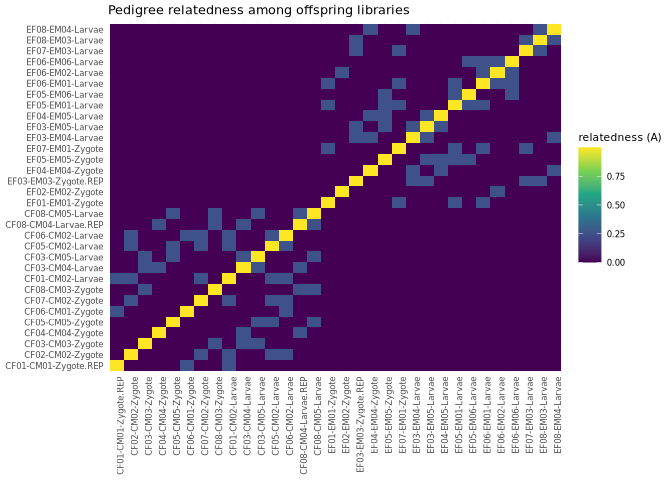
4 PQLseq2: binomial mixed model for parental-treatment effect
Fit, per CpG, a binomial mixed model:
meth_i / total_i ~ Binomial(total_i, p_i), logit(p_i) = intercept + treatment_i + stage_i + u_i, u ~ N(0, h2 * K)
- Predictor tested (
x) = parentaltreatment(Control = 0, Exposed = 1). - Covariate adjusted for (
W) =stage(Zygote = 0, Larvae = 1). PQLseq2 fits its own intercept, soWholds covariates only. - Random-effect covariance (
K) = the pedigree relatedness matrix.
Runs kept failing due to single sites throwing solve() errors and, while these only repesent fit failures for single CpG sites, the error kills the entire run. This should hopefully be addressed by the within-group filtering added above, but to make double sure I’m adding a wrapper tot he pqlseq2() function that essentially parses the full set of sites in chunks, and retries failed chunks in small batches. Ultimately, this should function to eaxclude failed sites from the run, rather than letting them corrupt/kill the whole job. Will also check, though, for how many sites ended up being dropped (high # could indicate lingering data preprocessing issues)
(utills::capture.output() added bc first successful run had thousands of lines of output messages about # of sites, chunks, etc.)
run_pqlseq2_safe <- function(Y, x, K, W, lib_size, chunk = 1000, ncores = 8, ...) {
  idx_chunks <- split(seq_len(nrow(Y)), ceiling(seq_len(nrow(Y)) / chunk))
  out <- vector("list", length(idx_chunks))
  for (i in seq_along(idx_chunks)) {
    rows <- idx_chunks[[i]]
    utils::capture.output(
    res  <- try(pqlseq2(Y = Y[rows, , drop = FALSE], x = x, K = K, W = W,
                        lib_size = lib_size[rows, , drop = FALSE],
                        ncores = ncores, ...), silent = TRUE)
    )
    if (inherits(res, "try-error")) {
      # if a site in this chunk threw a fatal solve() error, redo it site-by-site
      # so the singular one is dropped but its chunk-mates are kept
      res <- dplyr::bind_rows(lapply(rows, function(r) {
        utils::capture.output(
        s <- try(pqlseq2(Y = Y[r, , drop = FALSE], x = x, K = K, W = W,
                         lib_size = lib_size[r, , drop = FALSE],
                         ncores = 1, ...), silent = TRUE)
        )
        if (inherits(s, "try-error")) NULL else s
      }))
    }
    out[[i]] <- res
  }
  dplyr::bind_rows(out)
}
treatment_num <- as.numeric(meta$treatment) - 1 # Control=0, Exposed=1
stage_num <- as.numeric(meta$stage) - 1 # Zygote=0, Larvae=1
fit_pql <- run_pqlseq2_safe(
Y = meth_mat, # q x n methylated counts (rownames = "chr_pos")
x = treatment_num, # predictor of interest (parental treatment)
K = K, # n x n pedigree relatedness -> random effect
W = cbind(stage = stage_num), # covariates (life stage)
lib_size = cov_mat, # q x n total coverage
chunk = 1000,
ncores = 8,
model = "BMM", # binomial mixed model (MACAU model)
filter = TRUE, # drop sites w/o >=2 individuals having counts>5 (should be redundant)
check_K = TRUE,
verbose = FALSE
)
# wrapper check: how much of the data was actually fittable?
n_in <- nrow(meth_mat); n_out <- nrow(fit_pql); n_conv <- sum(fit_pql$converged, na.rm = TRUE)
cat("sites into fit: ", n_in, "\n",
"sites returned: ", n_out, " (", round(100 * n_out / n_in, 1), "% survived fitting)\n",
"of those, converged: ", n_conv, " (", round(100 * n_conv / n_out, 1), "%)\n", sep = "")## sites into fit: 2148546
## sites returned: 2148546 (100% survived fitting)
## of those, converged: 1997127 (93%)head(fit_pql)## outcome n intercept se_intercept beta se_beta pvalue
## 1 NC_007175.2_49 31 -4.035420 0.3181180 0.2946013 0.4041593 0.46604839
## 2 NC_007175.2_50 31 -3.643355 0.4000642 0.3819395 0.6318924 0.54555277
## 3 NC_007175.2_51 32 -3.686781 0.3325835 -0.9784464 0.4904543 0.04604510
## 4 NC_007175.2_52 31 -4.572153 0.5797449 0.1587980 0.7907265 0.84083511
## 5 NC_007175.2_88 32 -3.623185 0.2072900 -0.7102227 0.3178756 0.02546472
## 6 NC_007175.2_89 32 -4.195998 0.2633442 0.4007804 0.3670981 0.27494171
## h2 sigma2 converged elapsed_time
## 1 0.0000000 0.3029549 TRUE 1.116125
## 2 0.0000000 0.3950827 TRUE 1.116296
## 3 1.0000000 0.4155439 TRUE 8.556898
## 4 0.0000000 0.9539051 TRUE 1.116428
## 5 0.0000000 0.1880950 TRUE 1.068336
## 6 0.6881588 0.3761060 TRUE 7.9269495 Results: call DMLs
pqlseq2() returns beta (logit-scale effect of exposure), se_beta, Wald pvalue, and h2 (variance explained by relatedness). Add a BH-FDR, keep converged fits, call DMLs at FDR < 0.05.
res <- fit_pql %>%
  as_tibble() %>%
  filter(as.logical(converged)) %>%
  mutate(padj = p.adjust(pvalue, method = "BH"),
         pos  = as.integer(str_extract(outcome, "[0-9]+$")),   # site id = "chr_pos"
         chr  = str_remove(outcome, "_[0-9]+$")) %>%
  arrange(pvalue)

dml <- filter(res, padj < 0.05)
cat("Converged sites tested:", nrow(res), "\n")
## Converged sites tested: 1997127cat("Treatment DMLs (FDR < 0.05):", nrow(dml), "\n")## Treatment DMLs (FDR < 0.05): 799cat(" hyper in exposed (beta > 0):", sum(dml$beta > 0), "\n")## hyper in exposed (beta > 0): 361cat(" hypo in exposed (beta < 0):", sum(dml$beta < 0), "\n")## hypo in exposed (beta < 0): 438head(dml)## # A tibble: 6 x 14
## outcome n intercept se_intercept beta se_beta pvalue h2 sigma2
## <chr> <int> <dbl> <dbl> <dbl> <dbl> <dbl> <dbl> <dbl>
## 1 NC_035783.1_~ 25 -1.16 0.329 -2.23 0.247 2.07e-19 NaN 0
## 2 NC_035783.1_~ 23 -1.24 0.367 -3.19 0.372 9.87e-18 0 0.0927
## 3 NC_035783.1_~ 25 -1.33 0.360 -2.75 0.323 1.40e-17 1 0.0574
## 4 NC_035783.1_~ 24 -1.34 0.352 -2.54 0.301 3.23e-17 1 0.0215
## 5 NC_035787.1_~ 25 1.64 0.502 2.42 0.302 1.20e-15 1 0.0462
## 6 NC_035783.1_~ 23 -1.66 0.448 -3.27 0.420 6.68e-15 0 0.179
## # i 5 more variables: converged <lgl>, elapsed_time <dbl>, padj <dbl>,
## # pos <int>, chr <chr>6 Save outputs
save_bed <- function(df, path, score_col) {
  if (is.null(df) || nrow(df) == 0) {
    file.create(path)
    message("save_bed: no rows for ", basename(path), " — wrote empty file.")
    return(invisible(NULL))
  }
  if (all(c("chr","start","end") %in% names(df))) {
    start <- df$start; end <- df$end
  } else if (all(c("chr","pos") %in% names(df))) {
    start <- df$pos - 1L; end <- df$pos
  } else {
    stop("save_bed: df lacks chr/start/end or chr/pos for ", basename(path))
  }
  score <- if (score_col %in% names(df)) df[[score_col]] else NA_real_
  bed <- data.frame(chr = df$chr, start = start, end = end, score = score)
  write.table(bed, path, quote = FALSE, sep = "\t", row.names = FALSE, col.names = FALSE)
}

write_tsv(res, "../output/11.1-diff-methyl-MACAU/pqlseq_treatment_test.tsv")
save_bed(dml, "../output/11.1-diff-methyl-MACAU/treatment_DML.bed", "beta")