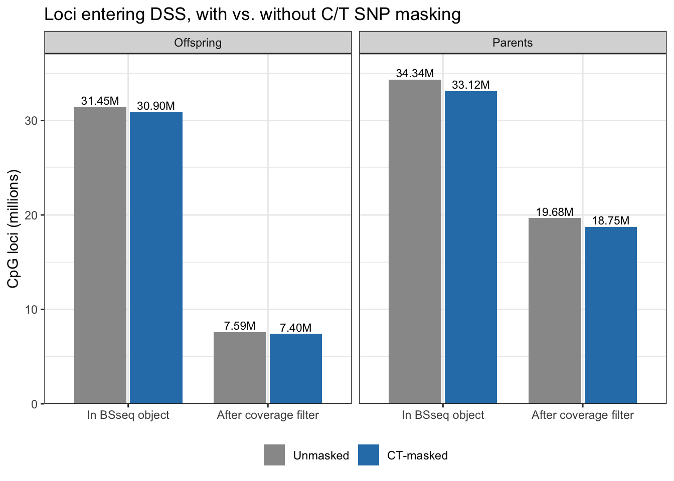
An important step of methylation analysis is excluding positions at which some individuals have C->T SNP variants, as this can lead to false-positive unmethylated cytosine calls.
I’d already called SNPs from the offspring data using BS-Snper at ceasmallr/code/12-snp-calling-BS-Snper.
I’ve now replicated the same code for use on the parent data at ceasmallr/code/12.1-snp-calling-BS-Snper-parents. For both .Rmd files, I’ve also added code to save a file of just C-T SNPs, for use with masking.
I then duplicated the scripts used to run DSS methylation analysis on both the offspring and parent data, adding a filtration step to remove C/T SNPs from the input .cov.gz files before loading as a BSseq object.
Full code can be found at: 10.01-diff-methyl-DSS-CTmask 10.11-diff-methyl-DSS-parents-CTmask
AI Disclosures:
Results
Comparing DSS outputs using unmasked and CT-SNP-masked datasets
Code
# Load packages library (dplyr)
Attaching package: 'dplyr'
The following objects are masked from 'package:stats':

    filter, lag
The following objects are masked from 'package:base':

    intersect, setdiff, setequal, union
Code
library (readr)library (stringr)library (tidyr)library (purrr)library (ggplot2)# Run from ceasmallr/code/ <- "../../../../ceasmallr/code" <- "../../../../ceasmallr/output" <- tribble (~ dataset, ~ masking, ~ md, ~ out,"Offspring" , "Unmasked" , "10-diff-methyl-DSS_remsamples.md" , "10-diff-methyl-DSS_remsamples" ,"Offspring" , "CT-masked" , "10.01-diff-methyl-DSS-CTmask.md" , "10.01-diff-methyl-DSS-CTmask" ,"Parents" , "Unmasked" , "10.1-diff-methyl-DSS-parents.md" , "10.1-diff-methyl-DSS-parents" ,"Parents" , "CT-masked" , "10.11-diff-methyl-DSS-parents-CTmask.md" , "10.11-diff-methyl-DSS-parents-CTmask" %>% mutate (masking = factor (masking, levels = c ("Unmasked" , "CT-masked" )))<- c ("Unmasked" = "grey60" , "CT-masked" = "#2C7FB8" )# ---- helpers ---------------------------------------------------------------- # Pull the first number from a knitted-output line ("## ...") matching `pattern` <- function (md_file, pattern) {<- read_lines (file.path (code_dir, md_file))<- str_match (lines, paste0 ("^ \\ s*## \\ s+" , pattern))[, 2 ]<- hit[! is.na (hit)]if (length (hit) == 0 ) return (NA_real_ )as.numeric (hit[1 ])# Count rows in a BED (empty file -> 0) <- function (path) {if (! file.exists (path) || file.size (path) == 0 ) return (0 L)length (read_lines (path))<- function (path, diff_name) {read_tsv (path, col_names = c ("chr" , "start" , "end" , diff_name), col_types = "ciid" )# ---- 1. Run-level summary values -------------------------------------------- <- runs %>% mutate (loci_bsseq = map_dbl (md, md_num, "( \\ d+) methylation loci" ),loci_retained = map_dbl (md, md_num, "Loci retained after coverage filter: ( \\ d+)" ),mf_trt_DML = map_dbl (md, md_num, "Treatment DMLs \\ (FDR < 0 \\ .05 \\ ): ( \\ d+)" ),mf_intx_DML = map_dbl (md, md_num, "Loci with (?:stage|sex)-dependent treatment effect \\ (FDR < 0 \\ .05 \\ ): ( \\ d+)" ),mf_trt_DMR = map_dbl (out, ~ bed_n (file.path (out_dir, .x, "treatment_DMR.bed" )))# ---- Plot 1: loci in BSseq object / retained after filter ------------------- <- run_summary %>% select (dataset, masking, loci_bsseq, loci_retained) %>% pivot_longer (c (loci_bsseq, loci_retained), names_to = "stage" , values_to = "n" ) %>% mutate (stage = recode (stage, loci_bsseq = "In BSseq object" ,loci_retained = "After coverage filter" ),stage = factor (stage, levels = c ("In BSseq object" , "After coverage filter" ))) %>% ggplot (aes (stage, n / 1e6 , fill = masking)) + geom_col (position = position_dodge (0.8 ), width = 0.75 ) + geom_text (aes (label = sprintf ("%.2fM" , n / 1e6 )),position = position_dodge (0.8 ), vjust = - 0.3 , size = 3 ) + facet_wrap (~ dataset) + scale_fill_manual (values = mask_cols) + scale_y_continuous (expand = expansion (mult = c (0 , 0.08 ))) + labs (x = NULL , y = "CpG loci (millions)" , fill = NULL ,title = "Loci entering DSS, with vs. without C/T SNP masking" ) + theme_bw () + theme (legend.position = "bottom" )
Code
# ---- Plot 2: multifactor results -------------------------------------------- <- run_summary %>% select (dataset, masking, mf_trt_DML, mf_intx_DML, mf_trt_DMR) %>% pivot_longer (starts_with ("mf_" ), names_to = "result" , values_to = "n" ) %>% mutate (result = recode (result,mf_trt_DML = "Treatment DMLs \n (FDR < 0.05)" ,mf_intx_DML = "Interaction DMLs \n (stage/sex-dependent)" ,mf_trt_DMR = "Treatment DMRs" )) %>% ggplot (aes (result, n, fill = masking)) + geom_col (position = position_dodge (0.8 ), width = 0.75 ) + geom_text (aes (label = scales:: comma (n)),position = position_dodge (0.8 ), vjust = - 0.3 , size = 3 ) + facet_wrap (~ dataset, scales = "free_y" ) + scale_fill_manual (values = mask_cols) + scale_y_continuous (labels = scales:: comma, expand = expansion (mult = c (0 , 0.1 ))) + labs (x = NULL , y = "Count" , fill = NULL ,title = "Multifactor DSS model (~ treatment + stage/sex [+ interaction])" ) + theme_bw () + theme (legend.position = "bottom" )
Code
# ---- Plot 3: within-stage / within-sex smoothed tests ----------------------- <- tribble (~ dataset, ~ group, ~ prefix,"Offspring" , "Zygote" , "zygote" ,"Offspring" , "Larvae" , "larvae" ,"Parents" , "Egg" , "female" ,"Parents" , "Sperm" , "male" <- runs %>% select (dataset, masking, out) %>% inner_join (group_files, by = "dataset" , relationship = "many-to-many" ) %>% mutate (DMLs = map2_int (out, prefix, ~ bed_n (file.path (out_dir, .x, paste0 (.y, "_DML.bed" )))),DMRs = map2_int (out, prefix, ~ bed_n (file.path (out_dir, .x, paste0 (.y, "_DMR.bed" ))))) %>% select (dataset, masking, group, DMLs, DMRs)<- group_counts %>% pivot_longer (c (DMLs, DMRs), names_to = "type" , values_to = "n" ) %>% mutate (group = factor (group, levels = c ("Zygote" , "Larvae" , "Egg" , "Sperm" ))) %>% ggplot (aes (group, n, fill = masking)) + geom_col (position = position_dodge (0.8 ), width = 0.75 ) + geom_text (aes (label = scales:: comma (n)),position = position_dodge (0.8 ), vjust = - 0.3 , size = 2.8 ) + facet_wrap (~ type, scales = "free_y" ) + scale_fill_manual (values = mask_cols) + scale_y_continuous (labels = scales:: comma, expand = expansion (mult = c (0 , 0.1 ))) + labs (x = NULL , y = "Count" , fill = NULL ,title = "Within-stage / within-sex smoothed DMLtest (exposed vs. control)" ) + theme_bw () + theme (legend.position = "bottom" )
Code
# ---- Plot 4: parent-offspring (and within-generation) DML overlaps ---------- # Recomputed from the DML BEDs so both versions use matching inputs: # Unmasked = 10-diff-methyl-DSS_remsamples offspring x 10.1 parents # CT-masked = 10.01 offspring x 10.11 parents <- function (off_out, par_out) {list (zyg = read_dml (file.path (out_dir, off_out, "zygote_DML.bed" ), "zyg_diff" ),lar = read_dml (file.path (out_dir, off_out, "larvae_DML.bed" ), "lar_diff" ),egg = read_dml (file.path (out_dir, par_out, "female_DML.bed" ), "egg_diff" ),sperm = read_dml (file.path (out_dir, par_out, "male_DML.bed" ), "sperm_diff" )<- c ("chr" , "start" , "end" )# every 2- and 3-way combination of DML sets; concordant = all diffs share one sign <- function (d) {<- unlist (lapply (2 : 3 , function (k) combn (names (d), k, simplify = FALSE )), recursive = FALSE )map_dfr (combs, function (cmb) {<- reduce (d[cmb], inner_join, by = by_loc)<- sign (as.matrix (j[, paste0 (cmb, "_diff" ), drop = FALSE ]))tibble (comparison = paste (cmb, collapse = " x " ),n_sets = length (cmb),n_shared = nrow (j),n_concordant = sum (apply (s, 1 , function (r) length (unique (r)) == 1 )))<- bind_rows (overlap_stats (load_dmls ("10-diff-methyl-DSS_remsamples" , "10.1-diff-methyl-DSS-parents" )) %>% mutate (masking = "Unmasked" ),overlap_stats (load_dmls ("10.01-diff-methyl-DSS-CTmask" , "10.11-diff-methyl-DSS-parents-CTmask" )) %>% mutate (masking = "CT-masked" )%>% mutate (masking = factor (masking, levels = c ("Unmasked" , "CT-masked" )),pct_concordant = 100 * n_concordant / n_shared,type = case_when (comparison %in% c ("zyg x lar" , "egg x sperm" ) ~ "Within generation" ,== 2 ~ "Parent x offspring" ,TRUE ~ "Three-way" ),comparison = str_replace_all (comparison, c ("zyg" = "Zygote" , "lar" = "Larvae" ,"egg" = "Egg" , "sperm" = "Sperm" )))<- overlaps %>% mutate (type = factor (type, levels = c ("Parent x offspring" , "Three-way" , "Within generation" ))) %>% ggplot (aes (reorder (comparison, n_shared), n_shared, fill = masking)) + geom_col (position = position_dodge (0.8 ), width = 0.75 ) + geom_text (aes (label = sprintf ("%s (%.0f%%)" , scales:: comma (n_shared), pct_concordant)),position = position_dodge (0.8 ), hjust = - 0.1 , size = 2.6 ) + coord_flip () + facet_grid (type ~ ., scales = "free_y" , space = "free_y" ) + scale_fill_manual (values = mask_cols) + scale_y_continuous (labels = scales:: comma, expand = expansion (mult = c (0 , 0.25 ))) + labs (x = NULL , y = "Shared DMLs (exact CpG position)" , fill = NULL ,title = "DML overlaps, with vs. without C/T SNP masking" ,subtitle = "Label: n shared (% direction-concordant across all sets)" ) + theme_bw () + theme (legend.position = "bottom" )
Code
# ---- Combined table of percent change --------------------------------------- <- bind_rows (%>% select (dataset, masking, loci_bsseq, loci_retained, mf_trt_DML, mf_intx_DML, mf_trt_DMR) %>% pivot_longer (- c (dataset, masking), names_to = "metric" , values_to = "n" ),%>% pivot_longer (c (DMLs, DMRs), names_to = "type" , values_to = "n" ) %>% transmute (dataset, masking, metric = paste (group, type), n),%>% transmute (dataset = "Overlap" , masking, metric = comparison, n = n_shared)%>% pivot_wider (names_from = masking, values_from = n) %>% mutate (pct_change = 100 * (` CT-masked ` - Unmasked) / Unmasked):: kable (pct_change, digits = 1 , format.args = list (big.mark = "," ))
Offspring
loci_bsseq
31,450,950
30,896,191
-1.8
Offspring
loci_retained
7,594,836
7,403,330
-2.5
Offspring
mf_trt_DML
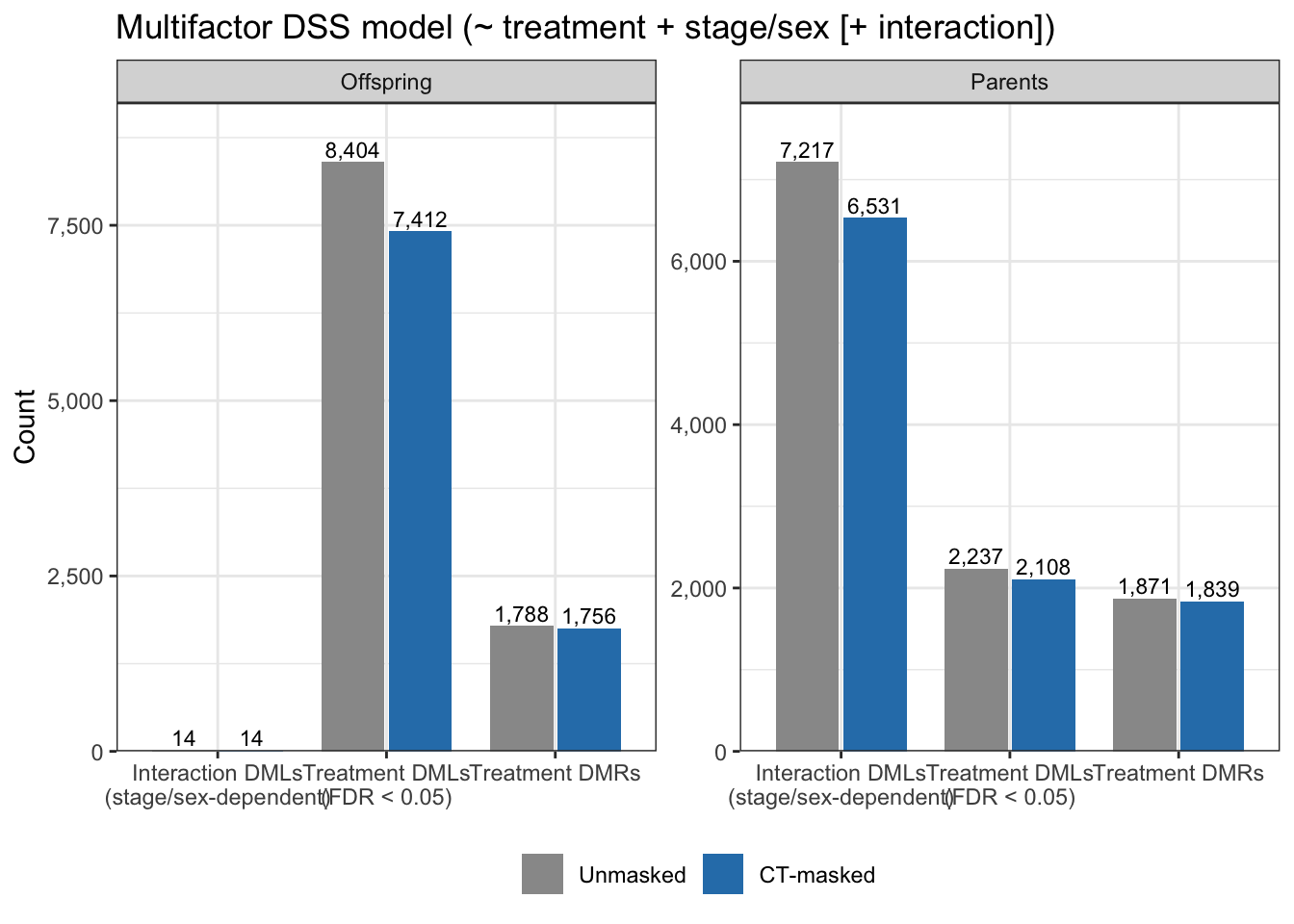
8,404
7,412
-11.8
Offspring
mf_intx_DML
14
14
0.0
Offspring
mf_trt_DMR
1,788
1,756
-1.8
Parents
loci_bsseq
34,343,214
33,122,286
-3.6
Parents
loci_retained
19,684,036
18,747,029
-4.8
Parents
mf_trt_DML
2,237
2,108
-5.8
Parents
mf_intx_DML
7,217
6,531
-9.5
Parents
mf_trt_DMR
1,871
1,839
-1.7
Offspring
Zygote DMLs
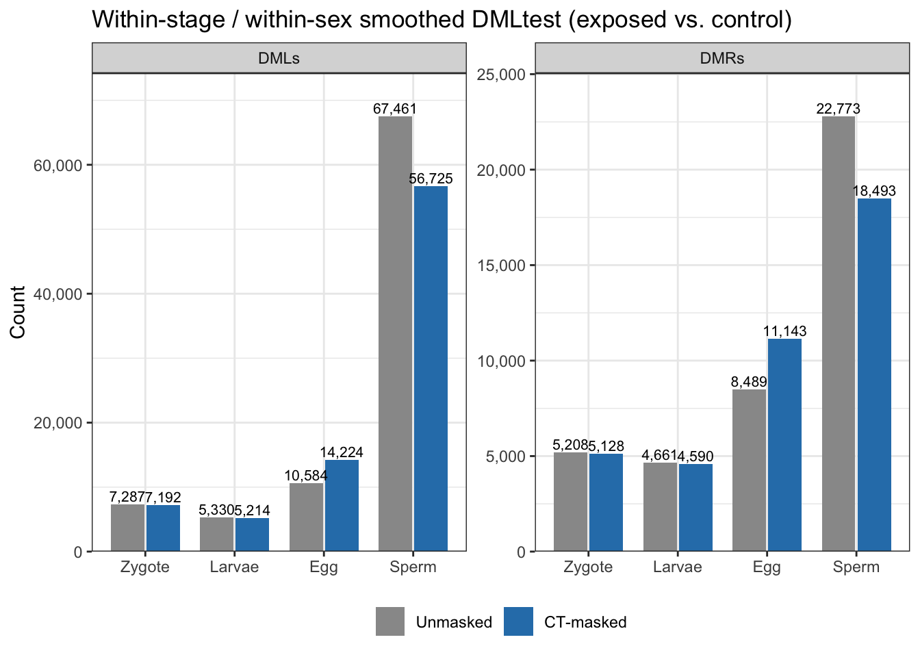
7,287
7,192
-1.3
Offspring
Zygote DMRs
5,208
5,128
-1.5
Offspring
Larvae DMLs
5,330
5,214
-2.2
Offspring
Larvae DMRs
4,661
4,590
-1.5
Parents
Egg DMLs
10,584
14,224
34.4
Parents
Egg DMRs
8,489
11,143
31.3
Parents
Sperm DMLs
67,461
56,725
-15.9
Parents
Sperm DMRs
22,773
18,493
-18.8
Overlap
Zygote x Larvae
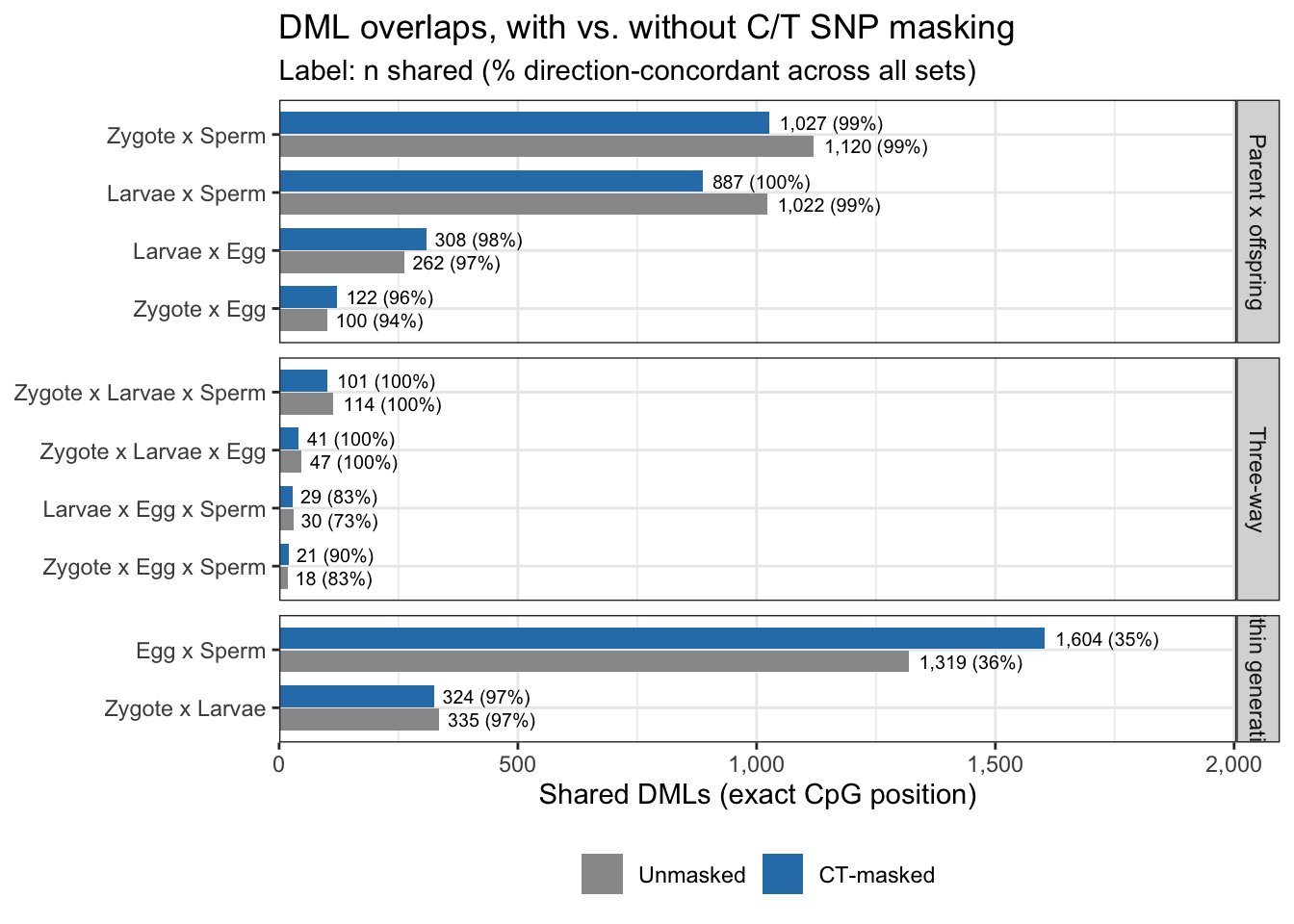
335
324
-3.3
Overlap
Zygote x Egg
100
122
22.0
Overlap
Zygote x Sperm
1,120
1,027
-8.3
Overlap
Larvae x Egg
262
308
17.6
Overlap
Larvae x Sperm
1,022
887
-13.2
Overlap
Egg x Sperm
1,319
1,604
21.6
Overlap
Zygote x Larvae x Egg
47
41
-12.8
Overlap
Zygote x Larvae x Sperm
114
101
-11.4
Overlap
Zygote x Egg x Sperm
18
21
16.7
Overlap
Larvae x Egg x Sperm
30
29
-3.3
More interesting is an instance where the CT-SNP-masked input led to an increaed # of identified features: From the parent data, within-sex tests found more DMLs and DMRs in the egg samples after masking
This isn’t too weird though. Masking C/T SNPs is expected to remove a portion of identified DMLs (e.g., SNP artifacts). However, one would also expect some “gains”, from loci whose signal was being hidden by nearby SNPs.