In Part 1 I ran the ML model on phenotype as a predictor of gene/miRNA expression.

This time I ran the ML model with miRNA expression as the predictor and gene expression as response to investigate miRNA-mRNA interactions. Note that, due to the high number of genes, I performed dimensionality reduction, essentially summarizing genes to PCs of coexpression

Results

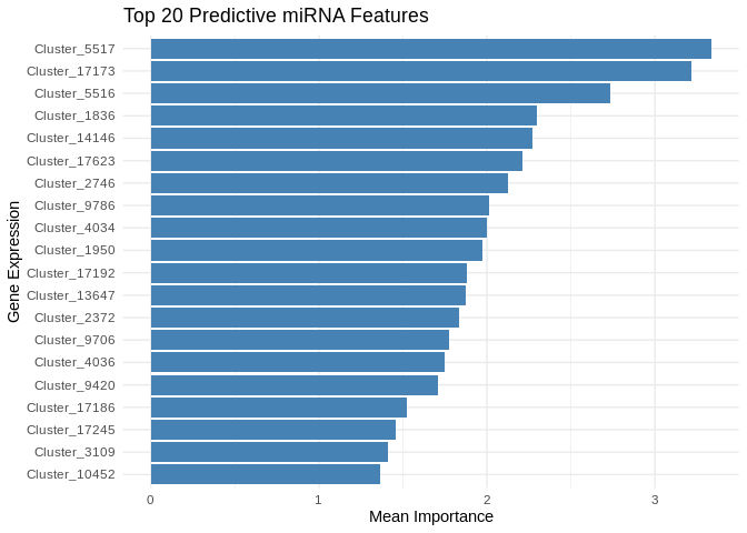
A couple miRNA pop out as notably highly predictive of gene expression, but all of the top 20 miRNA are important

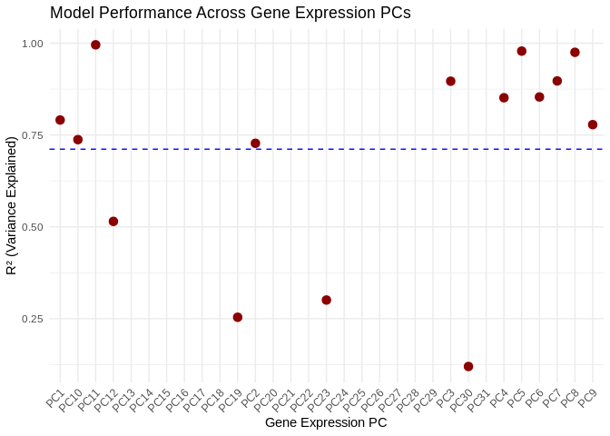
Many gene PCs are highly explained by miRNA expression, with 11 gene PCs of R² >~0.75

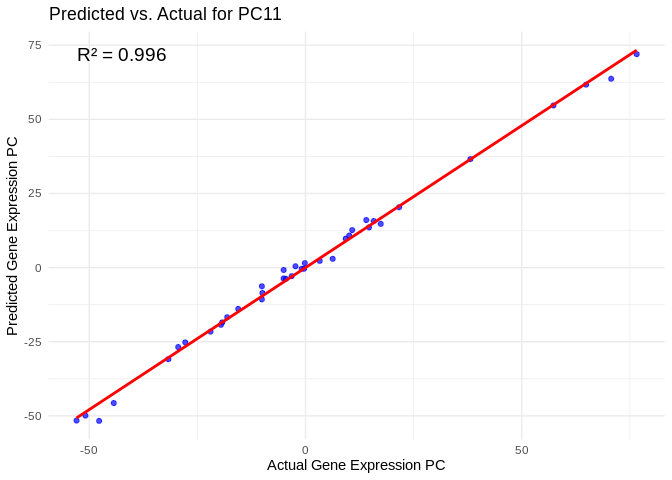
We can then look at which genes are included in highly predicted PCs. For example, in PC11, the most highly predicted PC, we see an R² of 0.996 and extremely strong model performance

Here are the top 20 genes included in PC11:

## # A tibble: 20 × 3
## # Groups:   Genes_PC [1]
##    gene       Genes_PC Loading
##    <chr>      <chr>      <dbl>
##  1 FUN_029347 PC11      0.0196
##  2 FUN_001854 PC11     -0.0193
##  3 FUN_025457 PC11      0.0192
##  4 FUN_021609 PC11     -0.0190
##  5 FUN_041974 PC11      0.0190
##  6 FUN_008614 PC11      0.0190
##  7 FUN_001958 PC11      0.0189
##  8 FUN_033958 PC11      0.0189
##  9 FUN_000394 PC11     -0.0188
## 10 FUN_039508 PC11      0.0187
## 11 FUN_016324 PC11     -0.0187
## 12 FUN_001244 PC11     -0.0185
## 13 FUN_016966 PC11     -0.0185
## 14 FUN_004574 PC11      0.0183
## 15 FUN_011795 PC11     -0.0181
## 16 FUN_015171 PC11      0.0181
## 17 FUN_009743 PC11      0.0180
## 18 FUN_039139 PC11      0.0180
## 19 FUN_020597 PC11      0.0180
## 20 FUN_032877 PC11      0.0180

We can also look at which miRNA most contributed to predicting expression for PC11

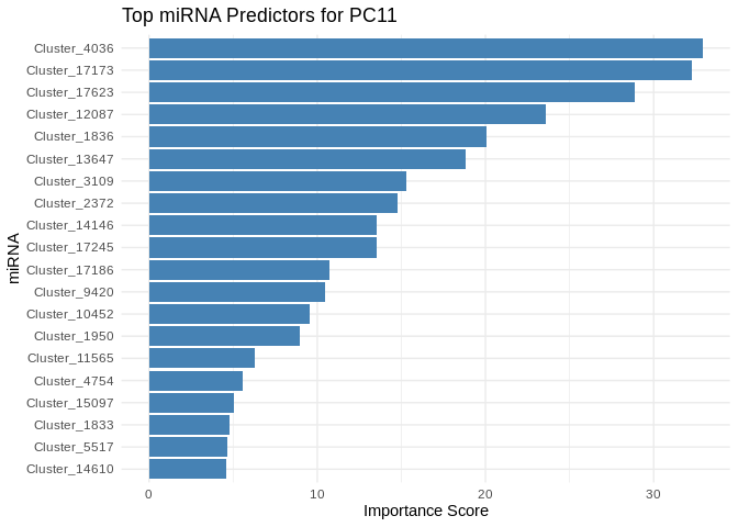We see that, rather than a single miRNA being primarily responsible for predicting PC11 expression, many are involved with high importance, suggesting a complex interaction network

Code copied below in case of file path changes:

I’d like to see whether phenotype can predict gene and/or miRNA expression, will be testing this using the ML approach Ariana has been trialing (see her mRNA-WGBS ML post here: https://ahuffmyer.github.io/ASH_Putnam_Lab_Notebook/E5-timeseries-molecular-mRNA-WGBS-machine-learning-analysis-Part-1/)

Inputs:

RNA counts matrix (raw): ../output/02.20-D-Apul-RNAseq-alignment-HiSat2/apul-gene_count_matrix.csv
sRNA/miRNA counts matrix (raw): ../output/03.10-D-Apul-sRNAseq-expression-DESeq2/Apul_miRNA_ShortStack_counts_formatted.txt
sample metadata: ../../M-multi-species/data/rna_metadata.csv
physiological data: https://github.com/urol-e5/timeseries/raw/refs/heads/master/time_series_analysis/Output/master_timeseries.csv

Note that I’ll start by using phenotype (e.g. biomass, respiration) as the predictor, which is suitable for understanding how external factors drive gene expression changes.

If, instead, we wanted to build some sort of predictive model, where gene expression could be used to predict phenotype, we could switch so that gene counts are used as the predictors.

Load libraries

library(tidyverse)
library(ggplot2)
library(DESeq2)
library(igraph)
library(psych)
library(tidygraph)
library(ggraph)
library(WGCNA)
library(edgeR)
library(reshape2)
library(ggcorrplot)
library(corrplot)
library(rvest)
library(purrr)
library(pheatmap)
library(glmnet)
library(caret)
library(factoextra)
library(vegan)
library(ggfortify)

Load and prep data

Load in count matrices for RNAseq.

# raw gene counts data (will filter and variance stabilize)
Apul_genes <- read_csv("../output/02.20-D-Apul-RNAseq-alignment-HiSat2/apul-gene_count_matrix.csv")
Apul_genes <- as.data.frame(Apul_genes)

# format gene IDs as rownames (instead of a column)
rownames(Apul_genes) <- Apul_genes$gene_id
Apul_genes <- Apul_genes%>%select(!gene_id)


# load and format metadata
metadata <- read_csv("../../M-multi-species/data/rna_metadata.csv")%>%select(AzentaSampleName, ColonyID, Timepoint) %>%
  filter(grepl("ACR", ColonyID))
metadata$Sample <- paste(metadata$AzentaSampleName, metadata$ColonyID, metadata$Timepoint, sep = "_")

colonies <- unique(metadata$ColonyID)

# Load physiological data
phys<-read_csv("https://github.com/urol-e5/timeseries/raw/refs/heads/master/time_series_analysis/Output/master_timeseries.csv")%>%filter(colony_id_corr %in% colonies)%>%
  select(colony_id_corr, species, timepoint, site, Host_AFDW.mg.cm2, Sym_AFDW.mg.cm2, Am, AQY, Rd, Ik, Ic, calc.umol.cm2.hr, cells.mgAFDW, prot_mg.mgafdw, Ratio_AFDW.mg.cm2, Total_Chl, Total_Chl_cell, cre.umol.mgafdw)
# format timepoint
phys$timepoint <- gsub("timepoint", "TP", phys$timepoint)
#add column with full sample info
phys <- merge(phys, metadata, by.x = c("colony_id_corr", "timepoint"), by.y = c("ColonyID", "Timepoint")) %>%
  select(-AzentaSampleName)
  

#add site information into metadata 
metadata$Site<-phys$site[match(metadata$ColonyID, phys$colony_id_corr)]


# Rename gene column names to include full sample info (as in miRNA table)
colnames(Apul_genes) <- metadata$Sample[match(colnames(Apul_genes), metadata$AzentaSampleName)]

# raw miRNA counts (will filter and variance stabilize)
Apul_miRNA <- read.table(file = "../output/03.10-D-Apul-sRNAseq-expression-DESeq2/Apul_miRNA_ShortStack_counts_formatted.txt", header = TRUE, sep = "\t", check.names = FALSE)

Counts filtering

Ensure there are no genes or miRNAs with 0 counts across all samples.

nrow(Apul_genes)

Apul_genes_filt<-Apul_genes %>%
     mutate(Total = rowSums(.[, 1:40]))%>%
    filter(!Total==0)%>%
    dplyr::select(!Total)

nrow(Apul_genes_filt)

# miRNAs
nrow(Apul_miRNA)

Apul_miRNA_filt<-Apul_miRNA %>%
     mutate(Total = rowSums(.[, 1:40]))%>%
    filter(!Total==0)%>%
    dplyr::select(!Total)

nrow(Apul_miRNA_filt)

Removing genes with only 0 counts reduced number from 44371 to 35869. Retained all 51 miRNAs.

Will not be performing pOverA filtering for now, since LM should presumabily incorporate sample representation

Physiology filtering

Run PCA on physiology data to see if there are phys outliers

Export data for PERMANOVA test.

test<-as.data.frame(phys)
test<-test[complete.cases(test), ]

Build PERMANOVA model.

scaled_test <-prcomp(test%>%select(where(is.numeric)), scale=TRUE, center=TRUE)
fviz_eig(scaled_test)

# scale data
vegan <- scale(test%>%select(where(is.numeric)))

# PerMANOVA 
permanova<-adonis2(vegan ~ timepoint*site, data = test, method='eu')
permanova

pca1<-ggplot2::autoplot(scaled_test, data=test, frame.colour="timepoint", loadings=FALSE,  colour="timepoint", shape="site", loadings.label.colour="black", loadings.colour="black", loadings.label=FALSE, frame=FALSE, loadings.label.size=5, loadings.label.vjust=-1, size=5) + 
  geom_text(aes(x = PC1, y = PC2, label = paste(colony_id_corr, timepoint)), vjust = -0.5)+
  theme_classic()+
   theme(legend.text = element_text(size=18), 
         legend.position="right",
        plot.background = element_blank(),
        legend.title = element_text(size=18, face="bold"), 
        axis.text = element_text(size=18), 
        axis.title = element_text(size=18,  face="bold"));pca1

Remove ACR-173, timepoint 3 sample from analysis. This is Azenta sample 1B2.

Apul_genes_filt <- Apul_genes_filt %>%
  select(!`1B2_ACR-173_TP3`)

Apul_miRNA_filt <- Apul_miRNA_filt %>%
  select(!`1B2_ACR-173_TP3`)

metadata <- metadata %>%
  filter(Sample != "1B2_ACR-173_TP3")

We also do not have phys data for colony 1B9 ACR-265 at TP4, so I’ll remove that here as well.

Apul_genes_filt <- Apul_genes_filt%>%
  select(!`1B9_ACR-265_TP4`)

Apul_miRNA_filt <- Apul_miRNA_filt%>%
  select(!`1B9_ACR-265_TP4`)

metadata <- metadata %>%
  filter(Sample != "1B9_ACR-265_TP4")

Assign metadata and arrange order of columns

Order metadata the same as the column order in the gene matrix.

list<-colnames(Apul_genes_filt)
list<-as.factor(list)

metadata$Sample<-as.factor(metadata$Sample)

# Re-order the levels
metadata$Sample <- factor(as.character(metadata$Sample), levels=list)
# Re-order the data.frame
metadata_ordered <- metadata[order(metadata$Sample),]
metadata_ordered$Sample

# Make sure the miRNA colnames are also in the same order as the gene colnames
Apul_miRNA_filt <- Apul_miRNA_filt[, colnames(Apul_genes_filt)]

Metadata and gene count matrix are now ordered the same.

Conduct variance stabilized transformation

VST should be performed on our two input datasets (gene counts and miRNA counts) separately

Genes:

#Set DESeq2 design
dds_genes <- DESeqDataSetFromMatrix(countData = Apul_genes_filt,
                              colData = metadata_ordered,
                              design = ~Timepoint+ColonyID)

Check size factors.

SF.dds_genes <- estimateSizeFactors(dds_genes) #estimate size factors to determine if we can use vst  to transform our data. Size factors should be less than 4 for us to use vst
print(sizeFactors(SF.dds_genes)) #View size factors

all(sizeFactors(SF.dds_genes)) < 4

All size factors are less than 4, so we can use VST transformation.

vsd_genes <- vst(dds_genes, blind=TRUE) #apply a variance stabilizing transformation to minimize effects of small counts and normalize with respect to library size
vsd_genes <- assay(vsd_genes)
head(vsd_genes, 3) #view transformed gene count data for the first three genes in the dataset.

miRNA:

#Set DESeq2 design
dds_miRNA <- DESeqDataSetFromMatrix(countData = Apul_miRNA_filt,
                              colData = metadata_ordered,
                              design = ~Timepoint+ColonyID)

Check size factors.

SF.dds_miRNA <- estimateSizeFactors(dds_miRNA) #estimate size factors to determine if we can use vst  to transform our data. Size factors should be less than 4 for us to use vst
print(sizeFactors(SF.dds_miRNA)) #View size factors

all(sizeFactors(SF.dds_miRNA)) < 4

All size factors are less than 4, so we can use VST transformation.

vsd_miRNA <- varianceStabilizingTransformation(dds_miRNA, blind=TRUE) #apply a variance stabilizing transformation to minimize effects of small counts and normalize with respect to library size. Using varianceStabilizingTransformation() instead of vst() because few input genes
vsd_miRNA <- assay(vsd_miRNA)
head(vsd_miRNA, 3) #view transformed gene count data for the first three genes in the dataset.

Combine counts data

# Extract variance stabilized counts as dataframes
# want samples in rows, genes/miRNAs in columns
vsd_genes <- as.data.frame(t(vsd_genes))
vsd_miRNA <- as.data.frame(t(vsd_miRNA))

# Double check the row names (sample names) are in same order
rownames(vsd_genes) == rownames(vsd_miRNA)

# Combine vst gene counts and vst miRNA counts by rows (sample names)
vsd_merged <- cbind(vsd_genes, vsd_miRNA)

Feature selection

Genes + miRNA

We have a large number of genes, so we’ll reduce dimensionality using PCA. Note that, since we only have a few phenotypes of interest, we don’t need to reduce this dataset

First need to remove any genes/miRNA that are invariant

vsd_merged_filt <- vsd_merged[, apply(vsd_merged, 2, var) > 0]

ncol(vsd_merged)
ncol(vsd_merged_filt)

colnames(vsd_merged[, apply(vsd_merged, 2, var) == 0])

Removed 74 invariant genes. I was worried we lost miRNA, but it looks like everything removed was a gene (prefix “FUN”)!

Reduce dimensionality (genes+miRNA)

# Perform PCA on gene+miRNA expression matrix
pca_merged <- prcomp(vsd_merged_filt, scale. = TRUE)

# Select top PCs that explain most variance (e.g., top 50 PCs)
explained_var <- summary(pca_merged)$importance[2, ]  # Cumulative variance explained
num_pcs <- min(which(cumsum(explained_var) > 0.95))  # Keep PCs that explain 95% variance

merged_pcs <- as.data.frame(pca_merged$x[, 1:num_pcs])  # Extract selected PCs

dim(merged_pcs)

We have 27 gene/miRNA expression PCs

Genes only

To investigate gene expression separately from miRNA expression, reduce dimensionality of genes alone.

Remove any genes that are invariant

vsd_genes_filt <- vsd_genes[, apply(vsd_genes, 2, var) > 0]

ncol(vsd_genes)
ncol(vsd_genes_filt)

Removed 74 invariant genes.

Reduce dimensionality

# Perform PCA on gene expression matrix
pca_genes <- prcomp(vsd_genes_filt, scale. = TRUE)

# Select top PCs that explain most variance (e.g., top 50 PCs)
explained_var_genes <- summary(pca_genes)$importance[2, ]  # Cumulative variance explained
num_pcs_genes <- min(which(cumsum(explained_var_genes) > 0.95))  # Keep PCs that explain 95% variance

genes_pcs <- as.data.frame(pca_genes$x[, 1:num_pcs_genes])  # Extract selected PCs

dim(genes_pcs)

Physiological metrics

Select physiological metrics of interest. For now we’ll focus on biomass (“Host_AFDW.mg.cm2”), protein (“prot_mg.mgafdw”), and respiration (“Rd”). These are all metrics of host energy storage and expenditure.

# Assign sample IDs to row names
rownames(phys) <- phys$Sample

# Select metrics
phys_selection <- phys %>% select(Host_AFDW.mg.cm2, prot_mg.mgafdw, Rd)

# Make sure the phys rownames are in the same order as the gene/miRNA rownames
phys_selection <- phys_selection[rownames(merged_pcs),]

Phenotype to predict gene/miRNA expression

The model

Train elastic models to predict gene expression PCs from phys data.

train_models <- function(response_pcs, predictor_pcs) {
  models <- list()
  
  for (pc in colnames(response_pcs)) {
    y <- response_pcs[[pc]]  # Gene expression PC
    X <- as.matrix(predictor_pcs)  # Phys as predictors
    
    # Train elastic net model (alpha = 0.5 for mix of LASSO & Ridge)
    model <- cv.glmnet(X, y, alpha = 0.5)
    
    models[[pc]] <- model
  }
  
  return(models)
}

# Train models predicting gene expression PCs from phys data
models <- train_models(merged_pcs, phys_selection)

Extract feature importance.

get_feature_importance <- function(models) {
  importance_list <- lapply(models, function(model) {
    coefs <- as.matrix(coef(model, s = "lambda.min"))[-1, , drop = FALSE]  # Convert to regular matrix & remove intercept
    
    # Convert to data frame
    coefs_df <- data.frame(Feature = rownames(coefs), Importance = as.numeric(coefs))
    
    return(coefs_df)
  })
  
  # Combine feature importance across all predicted gene PCs
  importance_df <- bind_rows(importance_list) %>%
    group_by(Feature) %>%
    summarize(MeanImportance = mean(abs(Importance)), .groups = "drop") %>%
    arrange(desc(MeanImportance))
  
  return(importance_df)
}

feature_importance <- get_feature_importance(models)
head(feature_importance, 20)  # Top predictive phys features

Evaluate performance.

evaluate_model_performance <- function(models, response_pcs, predictor_pcs) {
  results <- data.frame(PC = colnames(response_pcs), R2 = NA)
  
  for (pc in colnames(response_pcs)) {
    y <- response_pcs[[pc]]
    X <- as.matrix(predictor_pcs)
    
    model <- models[[pc]]
    preds <- predict(model, X, s = "lambda.min")
    
    R2 <- cor(y, preds)^2  # R-squared metric
    results[results$PC == pc, "R2"] <- R2
  }
  
  return(results)
}

performance_results <- evaluate_model_performance(models, merged_pcs, phys_selection)
summary(performance_results$R2)

Results

Plot results.

# Select top 20 predictive phys features
top_features <- feature_importance %>% top_n(20, MeanImportance)

# Plot
ggplot(top_features, aes(x = reorder(Feature, MeanImportance), y = MeanImportance)) +
  geom_bar(stat = "identity", fill = "steelblue") +
  coord_flip() +  # Flip for readability
  theme_minimal() +
  labs(title = "Top 20 Predictive Phys Features",
       x = "Physiological Metric",
       y = "Mean Importance")

ggplot(performance_results, aes(x = PC, y = R2)) +
  geom_point(color = "darkred", size = 3) +
  geom_hline(yintercept = mean(performance_results$R2, na.rm = TRUE), linetype = "dashed", color = "blue") +
  theme_minimal() +
  labs(title = "Model Performance Across Gene Expression PCs",
       x = "Gene Expression PC",
       y = "R² (Variance Explained)") +
  theme(axis.text.x = element_text(angle = 45, hjust = 1))  # Rotate labels

Keep in mind that, while we ran the model with physiological predictors, we’re really interested in the genes/miRNA associated with these predictors

View components associated with gene/miRNA PCs

# Get the PCA rotation (loadings) matrix from the original gene/miRNA PCA
merged_loadings <- pca_merged$rotation  # Each column corresponds to a PC

# Convert to data frame and reshape for plotting
merged_loadings_df <- as.data.frame(merged_loadings) %>%
  rownames_to_column(var = "gene_miRNA") %>%
  pivot_longer(-gene_miRNA, names_to = "Merged_PC", values_to = "Loading")

# View top CpGs contributing most to each PC
top_genes <- merged_loadings_df %>%
  group_by(Merged_PC) %>%
  arrange(desc(abs(Loading))) %>%
  slice_head(n = 20)  # Select top 10 CpGs per PC

print(top_genes)

View top 20 miRNA/genes associated with PC9 (the PC with the highest R^2)

print(top_genes%>%filter(Merged_PC=="PC9"))

Interesting, there’s an miRNA in there!

View predicted vs actual gene expression values to evaluate model.

# Choose a gene expression PC to visualize (e.g., the most predictable one)
best_pc <- performance_results$PC[which.max(performance_results$R2)]

# Extract actual and predicted values for that PC
actual_values <- merged_pcs[[best_pc]]
predicted_values <- predict(models[[best_pc]], as.matrix(phys_selection), s = "lambda.min")

# Create data frame
prediction_df <- data.frame(
  Actual = actual_values,
  Predicted = predicted_values
)

# Scatter plot with regression line
ggplot(prediction_df, aes(x = Actual, y = lambda.min)) +
  geom_point(color = "blue", alpha = 0.7) +
  geom_smooth(method = "lm", color = "red", se = FALSE) +
  theme_minimal() +
  labs(title = paste("Predicted vs. Actual for", best_pc),
       x = "Actual Gene Expression PC",
       y = "Predicted Gene Expression PC") +
  annotate("text", x = min(actual_values), y = max(predicted_values), 
           label = paste("R² =", round(max(performance_results$R2, na.rm=TRUE), 3)), 
           hjust = 0, color = "black", size = 5)
## `geom_smooth()` using formula = 'y ~ x'

miRNA expression to predict gene expression

The model

Train elastic models to predict gene expression PCs from phys data.

# Train models predicting gene expression PCs from phys data
models2 <- train_models(genes_pcs, vsd_miRNA)

Extract feature importance.

feature_importance2 <- get_feature_importance(models2)
head(feature_importance2, 20)  # Top predictive phys features

Evaluate performance.

performance_results2 <- evaluate_model_performance(models2, genes_pcs, vsd_miRNA)
summary(performance_results2$R2)

Results

Plot results.

# Select top 20 predictive phys features
top_features2 <- feature_importance2 %>% top_n(20, MeanImportance)

# Plot
ggplot(top_features2, aes(x = reorder(Feature, MeanImportance), y = MeanImportance)) +
  geom_bar(stat = "identity", fill = "steelblue") +
  coord_flip() +  # Flip for readability
  theme_minimal() +
  labs(title = "Top 20 Predictive miRNA Features",
       x = "Gene Expression",
       y = "Mean Importance")

ggplot(performance_results2, aes(x = PC, y = R2)) +
  geom_point(color = "darkred", size = 3) +
  geom_hline(yintercept = mean(performance_results2$R2, na.rm = TRUE), linetype = "dashed", color = "blue") +
  theme_minimal() +
  labs(title = "Model Performance Across Gene Expression PCs",
       x = "Gene Expression PC",
       y = "R² (Variance Explained)") +
  theme(axis.text.x = element_text(angle = 45, hjust = 1))  # Rotate labels

View components associated with gene PCs

# Get the PCA rotation (loadings) matrix from the original gene PCA
genes_loadings <- pca_genes$rotation  # Each column corresponds to a PC

# Convert to data frame and reshape for plotting
genes_loadings_df <- as.data.frame(genes_loadings) %>%
  rownames_to_column(var = "gene") %>%
  pivot_longer(-gene, names_to = "Genes_PC", values_to = "Loading")

# View top genes contributing most to each PC
top_genes2 <- genes_loadings_df %>%
  group_by(Genes_PC) %>%
  arrange(desc(abs(Loading))) %>%
  slice_head(n = 20)  # Select top 10 CpGs per PC

print(top_genes2)

View top 20 genes associated with PC11 (the most “predictable” PC, with the highest R^2)

print(top_genes2%>%filter(Genes_PC=="PC11"))

View predicted vs actual gene expression values to evaluate model.

# Choose a gene expression PC to visualize (e.g., the most predictable one)
best_pc2 <- performance_results2$PC[which.max(performance_results2$R2)]

# Extract actual and predicted values for that PC
actual_values2 <- genes_pcs[[best_pc2]]
predicted_values2 <- predict(models2[[best_pc2]], as.matrix(vsd_miRNA), s = "lambda.min")

# Create data frame
prediction_df2 <- data.frame(
  Actual = actual_values2,
  Predicted = predicted_values2
)

# Scatter plot with regression line
ggplot(prediction_df2, aes(x = Actual, y = lambda.min)) +
  geom_point(color = "blue", alpha = 0.7) +
  geom_smooth(method = "lm", color = "red", se = FALSE) +
  theme_minimal() +
  labs(title = paste("Predicted vs. Actual for", best_pc2),
       x = "Actual Gene Expression PC",
       y = "Predicted Gene Expression PC") +
  annotate("text", x = min(actual_values2), y = max(predicted_values2), 
           label = paste("R² =", round(max(performance_results2$R2, na.rm=TRUE), 3)), 
           hjust = 0, color = "black", size = 5)
## `geom_smooth()` using formula = 'y ~ x'

We can also look att which miRNA(s) contributed most to predicting gene PCs of interest

 get_feature_importance_for_pc <- function(model) {
  coefs <- as.matrix(coef(model, s = "lambda.min"))[-1, , drop = FALSE]  # Remove intercept
  coefs_df <- data.frame(Feature = rownames(coefs), Importance = abs(as.numeric(coefs)))
  
  return(coefs_df %>% arrange(desc(Importance)))  # Sort by importance
}

# Extract feature importance for the most predictable PC
#best_pc2 <- "PC11"
best_pc_model2 <- models2[[best_pc2]]
best_pc_importance2 <- get_feature_importance_for_pc(best_pc_model2)

# View top most important miRNA for predicting this PC
print(head(best_pc_importance2, 10))

# Plot
ggplot(best_pc_importance2 %>% head(20), aes(x = reorder(Feature, Importance), y = Importance)) +
  geom_bar(stat = "identity", fill = "steelblue") +
  coord_flip() +
  theme_minimal() +
  labs(title = paste("Top miRNA Predictors for", best_pc2),
       x = "miRNA",
       y = "Importance Score")