I originally ran MACAU with a very simple relatedness matrix created using the samples’ parent IDs, to essentially deliminate the half-sibs from everyone else. MACAU produced DML output, but the h2 values for almost all DMLs (h2 indicates heritability, or the portion of variance that can be attributed to relatedness) were stuck at the 0/1 bounds (see details here). This basically meant that the model couldn’t tell to what extent each site’s variation came from relatedness or from independent noise.
One of the data features that can cause this is collinearity between covariates – if relatedness overlaps with fixed effects (e.g., parental reatment condition), the fixed effect will obsorb the between-family differences, leaving little variance to be explained by relatedness. Generating a relatedness matrix manually from the parent IDs produced a relatedness matrix that was highly overlapping with parental treatment, since the offspring are stratified into either Control-only or Exposed-only parentage.
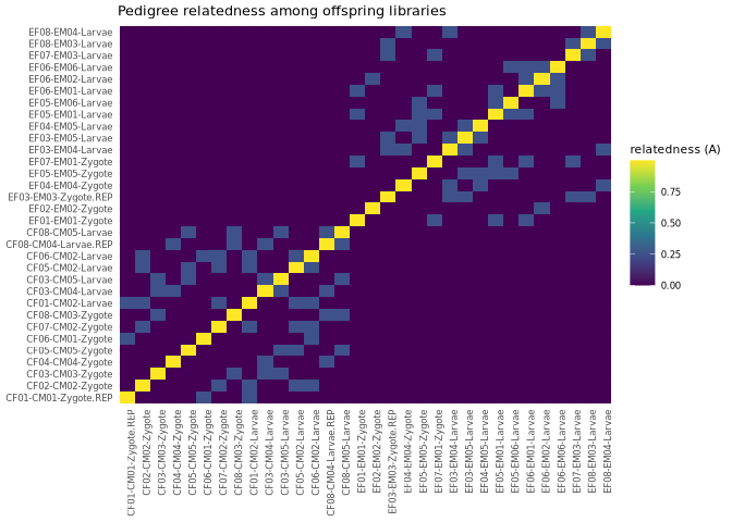
While this feature of the experimental design is unavoidable at this point, I can still try to generate a more accurate relatedness matrix that includes “background” relatedness values between all samples, not just the half-sibs. This can be done by doing SNP-calling on the WGBS data (using a tool that is bisulfite-aware, and won’t mistake C->T bisulfite conversions for genuine substitutions), then generating relatedness from that variant data. I’ve now done exactly that, using BS-Snper to call SNPs from the offspring WGBS data, then plink to generate a relatedness matrix from the output (see details here.
I will now rerun MACAU using this updated relatedness matrix to see if it improves ability to estimate heritability.
Results/Interpretation
Long story short, while MACAU still ran successfull and identified a similar number of parent-treatment-based DMLs, the h2 values were still largely bound to 0/1/NA, indicating the model is still unable to effectively parse variance attributable to relatedness. Moreover, the same proportion of DMLs produced non-0/1/NA h2 values – using the updated matrix, 44/624 (~7%) of DMLs had un-bound h2 values, while using the simplified matrix, 59/799 (~7%) did. This suggests to me that relatedness-treatment colinearity may not have been the (sole) underlying issue with effectively attributing site-level variance. It may also be related to the low sample size.
Full code available here and copied below
Code
Differential methylation analysis using MACAU, which has built-in functionality for incorporating informatin on population structure. This will help account for pseudoreplication in our ceasmallr samples stemming from shared parentage among the specimens.
As in 10-diff-methyl-DSS.Rmd and 10.1-diff-methyl-DSS-parents.Rmd, will need to run this .rmd using a .sh script on Klone (copy below for posterity)
#!/bin/bash
#SBATCH --account=srlab
#SBATCH --partition=cpu-g2-mem2x
#SBATCH --cpus-per-task=8
#SBATCH --mem=200G
#SBATCH --time=1-00:00:00
#SBATCH --output=macau_%j.out
#SBATCH --error=macau_%j.err
#SBATCH --chdir=/gscratch/srlab/kdurkin1/ceasmallr/code

apptainer exec --bind /gscratch:/gscratch \
 /gscratch/srlab/kdurkin1/srlab-R4.4-bioinformatics-container-703094b.sif \
  bash -c 'source /srlab/programs/miniforge3-24.7.1-0/etc/profile.d/conda.sh && conda activate /gscratch/srlab/kdurkin1/.conda/envs/macau && Rscript -e "rmarkdown::render(\"11.1-diff-methyl-MACAU-full-relat.Rmd\")"'
# Ended up needing to use PQLseq2 to implement the MACAU approach, instead of the MACAU 2.0 R package, which seemed to have some incompatabilites related to being built with an older version of R (?)
# PQLseq2 is also supported by MACAU authors (?)
library(PQLseq2)
library(bsseq)
library(BiocParallel)
library(nadiv)
library(readr)
library(dplyr)
library(stringr)
library(tibble)
library(ggplot2)
library(BiocParallel)1 Download methylation calls
(if necessary — same offspring files as used in 10-diff-methyl-DSS.Rmd)
wget \
--directory-prefix ../data/bismark-methyl-extraction \
--recursive \
--no-check-certificate \
--continue \
--cut-dirs 4 \
--no-host-directories \
--no-parent \
--quiet \
--no-clobber \
--accept="*.deduplicated.bismark.cov.gz,checksums.md5" https://gannet.fish.washington.edu/gitrepos/ceasmallr/output/02.20-bismark-methylation-extraction/
We should have N=32 (n=15 ControlxControl crosses, n=17 ExposedxExposed crosses)
2 Read Bismark coverage into a BSseq object
Same as 10-diff-methyl-DSS.Rmd: Bismark .cov columns (no header) are chr start end meth% count_methylated count_unmethylated; positions are 1-based. Read into a BSseq object so we get the union of CpG positions across samples, then pull the methylated-count and total-count matrices MACAU needs.
file.list  <- list.files("../data/bismark-methyl-extraction", pattern = "\\.bismark\\.cov\\.gz$", full.names = TRUE)

# As in 06.2, could drop the low-yield libraries (<100M Cs); leaving all in for now to maximize sample size
# drop <- c("CF01-CM01-Zygote", "CF08-CM04-Larvae", "CF08-CM05-Larvae", "EF04-EM04-Zygote", "EF05-EM05-Zygote")
# file.list <- file.list[!str_detect(basename(file.list), str_c(drop, collapse = "|"))]

# format sample IDs
sample.ids <- basename(file.list) %>%
  str_replace("_R1_001\\.fastp-trim_bismark_bt2_pe\\.deduplicated\\.bismark\\.cov\\.gz$", "") %>%
  str_replace("_R1_001\\.fastp-trim\\.REPAIRED_bismark_bt2_pe\\.deduplicated\\.bismark\\.cov\\.gz$", ".REP")

# Grab treatment and lifestage info from Sample IDs
#   first letter of the cross code = parental treatment (C = control, E = exposed)
#   stage encoded in the ID string (Zygote / Larvae)
meta <- tibble(
  sample    = sample.ids,
  file      = file.list,
  treatment = case_when(str_starts(sample.ids, "E") ~ "Exposed",
                        str_starts(sample.ids, "C") ~ "Control",
                        TRUE ~ NA_character_),
  stage     = case_when(str_detect(sample.ids, "Zygote") ~ "Zygote",
                        str_detect(sample.ids, "Larvae") ~ "Larvae",
                        TRUE ~ NA_character_)
) %>%
  # reference levels: Control (so the coefficient = effect of exposure) and Zygote (earlier stage)
  mutate(treatment = factor(treatment, levels = c("Control", "Exposed")),
         stage     = factor(stage,     levels = c("Zygote",  "Larvae")))

knitr::kable(count(meta, treatment, stage))| treatment | stage | n |
|---|---|---|
| Control | Zygote | 8 |
| Control | Larvae | 7 |
| Exposed | Zygote | 6 |
| Exposed | Larvae | 11 |
colData <- DataFrame(treatment = meta$treatment,
                     stage     = meta$stage,
                     row.names = meta$sample)

BSobj <- read.bismark(files          = meta$file,
                      colData        = colData,
                      rmZeroCov      = TRUE,          # drops positions covered in 0 samples
                      strandCollapse = FALSE,         # .cov isn't a cytosine report; leave off
                      BPPARAM        = MulticoreParam(workers = 12, progressbar = TRUE),
                      verbose        = TRUE)
## [read.bismark] Parsing files and constructing valid loci ...
## | | | 0% | |== | 3% | |===== | 6% | |======= | 10% | |========= | 13% | |=========== | 16% | |============== | 19% | |================ | 23% | |================== | 26% | |==================== | 29% | |======================= | 32% | |========================= | 35% | |=========================== | 39% | |============================= | 42% | |================================ | 45% | |================================== | 48% | |==================================== | 52% | |====================================== | 55% | |========================================= | 58% | |=========================================== | 61% | |============================================= | 65% | |=============================================== | 68% | |================================================== | 71% | |==================================================== | 74% | |====================================================== | 77% | |======================================================== | 81% | |=========================================================== | 84% | |============================================================= | 87% | |=============================================================== | 90% | |================================================================= | 94% | |==================================================================== | 97% | |======================================================================| 100%
## Done in 73.8 secs
## [read.bismark] Parsing files and constructing 'M' and 'Cov' matrices ...
## | | | 0% | |== | 3% | |==== | 6% | |======= | 9% | |========= | 12% | |=========== | 16% | |============= | 19% | |=============== | 22% | |================== | 25% | |==================== | 28% | |====================== | 31% | |======================== | 34% | |========================== | 38% | |============================ | 41% | |=============================== | 44% | |================================= | 47% | |=================================== | 50% | |===================================== | 53% | |======================================= | 56% | |========================================== | 59% | |============================================ | 62% | |============================================== | 66% | |================================================ | 69% | |================================================== | 72% | |==================================================== | 75% | |======================================================= | 78% | |========================================================= | 81% | |=========================================================== | 84% | |============================================================= | 88% | |=============================================================== | 91% | |================================================================== | 94% | |==================================================================== | 97% | |======================================================================| 100%
## Done in 28.8 secs
## [read.bismark] Constructing BSseq object ...BSobj # positions are the UNION across samples; missing positions get N = 0## An object of type 'BSseq' with
## 31596324 methylation loci
## 32 samples
## has not been smoothed
## All assays are in-memory# Require non-zero coverage in >= half the samples of each treatment x stage cell.
cov_check <- getCoverage(BSobj, type = "Cov")
cells <- interaction(meta$treatment, meta$stage, drop = TRUE)
keep <- Reduce(`&`, lapply(levels(cells), function(cl) {
idx <- which(cells == cl)
rowSums(cov_check[, idx, drop = FALSE] > 0) >= ceiling(length(idx) / 2)
}))
BSobj <- BSobj[keep, ]
cat("Loci retained after coverage filter:", nrow(BSobj), "\n")## Loci retained after coverage filter: 6337469# Separation-aware filter
# Was getting errors (fatal `solve(): solution not found`) related to within-group sites
# that were either all 0% or all 100%.
# To prevent, require enough covered samples AND both methylated and unmethylated signal.
# within each treatment group
Mmat <- getCoverage(BSobj, type = "M")
Cmat <- getCoverage(BSobj, type = "Cov")
Umat <- Cmat - Mmat
grp <- meta$treatment
# Can adjust these parameters if desired
ok <- sapply(levels(grp), function(g) {
j <- which(grp == g)
covered <- rowSums(Cmat[, j, drop = FALSE] >= 5) # samples with >=5x in this group
hasM <- rowSums(Mmat[, j, drop = FALSE] > 0) # samples with >=1 methylated read
hasU <- rowSums(Umat[, j, drop = FALSE] > 0) # samples with >=1 unmethylated read
(covered >= 3) & (hasM >= 2) & (hasU >= 2)
})
BSobj <- BSobj[ok[, "Control"] & ok[, "Exposed"], ]
cat("Loci retained after separation-aware filter:", nrow(BSobj), "\n")## Loci retained after separation-aware filter: 2148546Per-site mixed-model fitting is very slow across whole genome. As in the DSS workflow, add a test-run switch that thins loci for troubleshooting.
# Keeps all samples but randomly thins loci genome-wide.
# set test_run to FALSE for full-data runs
test_run  <- FALSE
test_frac <- 0.0002      # keep 2% of loci

if (test_run) {
  set.seed(1)
  idx   <- sort(sample(nrow(BSobj), size = floor(nrow(BSobj) * test_frac)))
  BSobj <- BSobj[idx, ]
  cat("TEST RUN — loci subsampled to:", nrow(BSobj), "\n")
}
Pull the two count matrices MACAU needs both methylated counts (X) and total coverage (N). Rows = loci, columns = samples, in the same sample order as meta.
gr       <- granges(BSobj)
site_ids <- paste0(as.character(seqnames(gr)), "_", start(gr))

meth_mat <- as.matrix(getCoverage(BSobj, type = "M"))    # methylated read counts
cov_mat  <- as.matrix(getCoverage(BSobj, type = "Cov"))  # total read counts (library size)
rownames(meth_mat) <- rownames(cov_mat) <- site_ids
colnames(meth_mat) <- colnames(cov_mat) <- meta$sample

# check columns line up
stopifnot(identical(colnames(meth_mat), meta$sample),
          identical(dim(meth_mat), dim(cov_mat)),
          all(meth_mat <= cov_mat))


cat("Count matrices:", nrow(meth_mat), "loci x", ncol(meth_mat), "samples\n")
## Count matrices: 2148546 loci x 32 samples3 Load relatedness matrix
This time, the relatedness matrix was generated using SNP variants called from the samples’ WGBS data using BS-Snper
# Genomic relatedness matrix (GRM) from BS-Snper SNPs, via PLINK --make-rel square
rel_dir <- "../output/12-snp-calling-BS-Snper/per-sample"

K_geno <- as.matrix(read.table(file.path(rel_dir, "relatedness.rel")))
# .rel.id has FID and IID columns (plus a "#FID IID" header in PLINK 2); IID is the sample name
rel_ids <- read.table(file.path(rel_dir, "relatedness.rel.id"),
                      comment.char = "#", colClasses = "character")$V2
dimnames(K_geno) <- list(rel_ids, rel_ids)

# Methylation sample IDs can carry a ".REP" suffix (repaired libraries); BAM-derived IDs don't
meth_key <- str_remove(meta$sample, "\\.REP$")

# Report any samples missing from either dataset
missing_geno <- meta$sample[!meth_key %in% rel_ids]
extra_geno   <- setdiff(rel_ids, meth_key)
if (length(missing_geno)) cat("In methylation data but not in GRM (dropped):",
                              paste(missing_geno, collapse = ", "), "\n")
if (length(extra_geno))   cat("In GRM but not in methylation data (ignored):",
                              paste(extra_geno, collapse = ", "), "\n")

# Keep only samples present in both, and put K in the same order as the count matrices
keep_samp <- meth_key %in% rel_ids
meta      <- meta[keep_samp, ]
meth_mat  <- meth_mat[, keep_samp, drop = FALSE]
cov_mat   <- cov_mat[,  keep_samp, drop = FALSE]
meth_key  <- meth_key[keep_samp]

K <- K_geno[meth_key, meth_key]
dimnames(K) <- list(meta$sample, meta$sample)

stopifnot(identical(rownames(K), colnames(meth_mat)),
          identical(colnames(meth_mat), colnames(cov_mat)),
          isSymmetric(K),
          !anyNA(K))

# The PLINK GRM is standardized (diagonal ~1, off-diagonals can be negative) and is not
# guaranteed to be positive definite. The mixed model needs it to be, so fix it if necessary.
min_eig <- min(eigen(K, symmetric = TRUE, only.values = TRUE)$values)
cat("Smallest eigenvalue of K:", signif(min_eig, 3), "\n")
## Smallest eigenvalue of K: -0.314if (min_eig <= 1e-8) {
K <- as.matrix(Matrix::nearPD(K, corr = FALSE, keepDiag = TRUE)$mat)
dimnames(K) <- list(meta$sample, meta$sample)
cat("K adjusted to nearest positive-definite matrix\n")
}## K adjusted to nearest positive-definite matrixcat("Samples in model:", ncol(K), "\n")## Samples in model: 32summary(K[upper.tri(K)])## Min. 1st Qu. Median Mean 3rd Qu. Max.
## -0.15689 -0.04182 -0.02982 -0.01523 -0.01084 0.35882Quick look at the relatedness structure (how much pseudoreplication are we actually modeling?):
# heatmap
ord <- order(meta$treatment, meta$stage)
as.data.frame(as.table(K[ord, ord])) %>%
  ggplot(aes(Var1, Var2, fill = Freq)) +
  geom_tile() +
  scale_fill_viridis_c(name = "relatedness (A)") +
  theme_minimal(base_size = 8) +
  theme(axis.text.x = element_text(angle = 90, hjust = 1)) +
  labs(x = NULL, y = NULL, title = "Pedigree relatedness among offspring libraries")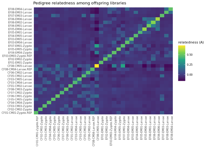
4 PQLseq2: binomial mixed model for parental-treatment effect
Fit, per CpG, a binomial mixed model:
meth_i / total_i ~ Binomial(total_i, p_i), logit(p_i) = intercept + treatment_i + stage_i + u_i, u ~ N(0, h2 * K)
- Predictor tested (
x) = parentaltreatment(Control = 0, Exposed = 1). - Covariate adjusted for (
W) =stage(Zygote = 0, Larvae = 1). PQLseq2 fits its own intercept, soWholds covariates only. - Random-effect covariance (
K) = the pedigree relatedness matrix.
Runs kept failing due to single sites throwing solve() errors and, while these only repesent fit failures for single CpG sites, the error kills the entire run. This should hopefully be addressed by the within-group filtering added above, but to make double sure I’m adding a wrapper tot he pqlseq2() function that essentially parses the full set of sites in chunks, and retries failed chunks in small batches. Ultimately, this should function to eaxclude failed sites from the run, rather than letting them corrupt/kill the whole job. Will also check, though, for how many sites ended up being dropped (high # could indicate lingering data preprocessing issues)
(utills::capture.output() added bc first successful run had thousands of lines of output messages about # of sites, chunks, etc.)
run_pqlseq2_safe <- function(Y, x, K, W, lib_size, chunk = 1000, ncores = 8, ...) {
  idx_chunks <- split(seq_len(nrow(Y)), ceiling(seq_len(nrow(Y)) / chunk))
  out <- vector("list", length(idx_chunks))
  for (i in seq_along(idx_chunks)) {
    rows <- idx_chunks[[i]]
    utils::capture.output(
    res  <- try(pqlseq2(Y = Y[rows, , drop = FALSE], x = x, K = K, W = W,
                        lib_size = lib_size[rows, , drop = FALSE],
                        ncores = ncores, ...), silent = TRUE)
    )
    if (inherits(res, "try-error")) {
      # if a site in this chunk threw a fatal solve() error, redo it site-by-site
      # so the singular one is dropped but its chunk-mates are kept
      res <- dplyr::bind_rows(lapply(rows, function(r) {
        utils::capture.output(
        s <- try(pqlseq2(Y = Y[r, , drop = FALSE], x = x, K = K, W = W,
                         lib_size = lib_size[r, , drop = FALSE],
                         ncores = 1, ...), silent = TRUE)
        )
        if (inherits(s, "try-error")) NULL else s
      }))
    }
    out[[i]] <- res
  }
  dplyr::bind_rows(out)
}
treatment_num <- as.numeric(meta$treatment) - 1 # Control=0, Exposed=1
stage_num <- as.numeric(meta$stage) - 1 # Zygote=0, Larvae=1
fit_pql <- run_pqlseq2_safe(
Y = meth_mat, # q x n methylated counts (rownames = "chr_pos")
x = treatment_num, # predictor of interest (parental treatment)
K = K, # n x n pedigree relatedness -> random effect
W = cbind(stage = stage_num), # covariates (life stage)
lib_size = cov_mat, # q x n total coverage
chunk = 1000,
ncores = 8,
model = "BMM", # binomial mixed model (MACAU model)
filter = TRUE, # drop sites w/o >=2 individuals having counts>5 (should be redundant)
check_K = TRUE,
verbose = FALSE
)
# wrapper check: how much of the data was actually fittable?
n_in <- nrow(meth_mat); n_out <- nrow(fit_pql); n_conv <- sum(fit_pql$converged, na.rm = TRUE)
cat("sites into fit: ", n_in, "\n",
"sites returned: ", n_out, " (", round(100 * n_out / n_in, 1), "% survived fitting)\n",
"of those, converged: ", n_conv, " (", round(100 * n_conv / n_out, 1), "%)\n", sep = "")## sites into fit: 2148546
## sites returned: 2148546 (100% survived fitting)
## of those, converged: 1997141 (93%)head(fit_pql)## outcome n intercept se_intercept beta se_beta pvalue h2
## 1 NC_007175.2_49 31 -4.035420 0.3181180 0.2946013 0.4041593 0.46604839 0
## 2 NC_007175.2_50 31 -3.643355 0.4000642 0.3819395 0.6318924 0.54555277 0
## 3 NC_007175.2_51 32 -3.719352 0.3009815 -0.9097625 0.4792840 0.05767369 1
## 4 NC_007175.2_52 31 -4.728423 0.5897950 0.1940027 0.8717852 0.82389740 1
## 5 NC_007175.2_88 32 -3.623185 0.2072900 -0.7102227 0.3178756 0.02546472 0
## 6 NC_007175.2_89 32 -4.144422 0.2448640 0.3671773 0.3922338 0.34921215 1
## sigma2 converged elapsed_time
## 1 0.3029549 TRUE 0.083449337
## 2 0.3950827 TRUE 0.083785234
## 3 0.7510785 TRUE 4.753266534
## 4 2.0747490 TRUE 0.001311016
## 5 0.1880950 TRUE 0.207945961
## 6 0.7990319 TRUE 5.5573920515 Results: call DMLs
pqlseq2() returns beta (logit-scale effect of exposure), se_beta, Wald pvalue, and h2 (variance explained by relatedness). Add a BH-FDR, keep converged fits, call DMLs at FDR < 0.05.
res <- fit_pql %>%
  as_tibble() %>%
  filter(as.logical(converged)) %>%
  mutate(padj = p.adjust(pvalue, method = "BH"),
         pos  = as.integer(str_extract(outcome, "[0-9]+$")),   # site id = "chr_pos"
         chr  = str_remove(outcome, "_[0-9]+$")) %>%
  arrange(pvalue)

dml <- filter(res, padj < 0.05)
cat("Converged sites tested:", nrow(res), "\n")
## Converged sites tested: 1997141cat("Treatment DMLs (FDR < 0.05):", nrow(dml), "\n")## Treatment DMLs (FDR < 0.05): 624cat(" hyper in exposed (beta > 0):", sum(dml$beta > 0), "\n")## hyper in exposed (beta > 0): 279cat(" hypo in exposed (beta < 0):", sum(dml$beta < 0), "\n")## hypo in exposed (beta < 0): 345head(dml)## # A tibble: 6 x 14
## outcome n intercept se_intercept beta se_beta pvalue h2 sigma2
## <chr> <int> <dbl> <dbl> <dbl> <dbl> <dbl> <dbl> <dbl>
## 1 NC_035783.1_~ 25 -1.16 0.329 -2.23 0.247 2.07e-19 NaN 0
## 2 NC_035783.1_~ 23 -1.24 0.367 -3.19 0.372 9.87e-18 0 0.0927
## 3 NC_035783.1_~ 25 -1.34 0.355 -2.74 0.320 1.03e-17 1 0.112
## 4 NC_035783.1_~ 24 -1.34 0.350 -2.54 0.300 2.26e-17 1 0.0406
## 5 NC_035787.1_~ 25 1.64 0.501 2.41 0.306 3.20e-15 1 0.100
## 6 NC_035783.1_~ 23 -1.66 0.448 -3.27 0.420 6.68e-15 0 0.179
## # i 5 more variables: converged <lgl>, elapsed_time <dbl>, padj <dbl>,
## # pos <int>, chr <chr>Breakdown of what each column represents:
n: The per-site sample size – for that site, how many individuals (out of 32) had coverage at this site and were used during model fittingintercept: baseline methylation for the reference group (Control, Zygote) on the logit scalese_intercept: SE of interecpt ^beta: DML effect – change in log-odds methylation, adjusted for lifestage and relatedness. Sign indicates direction (hyper-or hypo-methylated)se_beta: SE ofbeta^pvalue: Wald-test p-value (H_0 is beta=0, no treatment effect) – NOTE this is not corrected for multiple testing in default output, have to correct manuallyh2: heritability metric, fraction of latent variance assigned to relatedness – eaaentially, how much of methylation variance at the site is explained by pedigree. Highh2indicates signal at the DML is family-structuredsigma2: total variance component (kinship + residual)converged: did the model fit converge?elapsed_time: time required to fit the site
I’ve added:
padj: adjusted pvalue (BH, calculated frompvalue)pos/chrparsed genomic coordinates
NOTE that beta is a logit-scale log-odds, not a % methylation difference, so magnitudes are not directly comparable to methylation difference values produced by DSS or methylKit. I can still, however, compare direction (+/- to indicate hyper-/hypomethylation) and rank.
6 Save outputs
save_bed <- function(df, path, score_col) {
  if (is.null(df) || nrow(df) == 0) {
    file.create(path)
    message("save_bed: no rows for ", basename(path), " — wrote empty file.")
    return(invisible(NULL))
  }
  if (all(c("chr","start","end") %in% names(df))) {
    start <- df$start; end <- df$end
  } else if (all(c("chr","pos") %in% names(df))) {
    start <- df$pos - 1L; end <- df$pos
  } else {
    stop("save_bed: df lacks chr/start/end or chr/pos for ", basename(path))
  }
  score <- if (score_col %in% names(df)) df[[score_col]] else NA_real_
  bed <- data.frame(chr = df$chr, start = start, end = end, score = score)
  write.table(bed, path, quote = FALSE, sep = "\t", row.names = FALSE, col.names = FALSE)
}

write_tsv(res, "../output/11.1-diff-methyl-MACAU-full-relat/pqlseq_treatment_test.tsv")
save_bed(dml, "../output/11.1-diff-methyl-MACAU-full-relat/treatment_DML.bed", "beta")